Visualizing CES production functions with Wolfram Alpha

In this post, I will show how it is simple to visualize CES production functions with Wolfram Alpha. I build upon the very pedagogical YouTube video of Klaus Prettner on the basic properties of the neoclassical production function, available here: https://youtu.be/As40XvuMFOg

In his video, he recalls the basic properties of the CES production functions. I present the equations below:

• The constant elasticity of substitution (CES) production function is given by

Y=[\alpha K^\rho+(1-\alpha) L^\rho]^{\frac{\xi}{\rho}} 

Where α is the share of the two production factors in final output; ρ determines the substitutability between K and L in production; σ =1 /(1-ρ) is the elasticity of substitution between K and L; ξ denotes the returns to scale: ξ <1 : decreasing returns to scale, ξ >1 : increasing returns to scale, ξ =1 : constant returns to scale.

With constant returns to scale, we have

Y=[\alpha K^\rho+(1-\alpha) L^\rho]^{\frac{1}{\rho}} 

ρ ∈ (-∞,1] determines the elasticity of substitution:

• ρ → -∞: K and L are perfect complements ⇒ Leontief production function.
• ρ → 1: K and L are perfect substitutes ⇒ linear production function.
• ρ → 0: intermediate case in which K and L are imperfect substitutes ⇒ Cobb-Douglas production function.

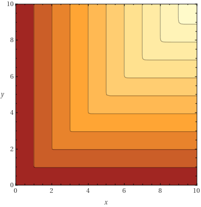
Now, I will show how to plot each case using Wolfram Alpha. We start with Leontief production function. You have to go to the Wolfram Alpha website and enter one of the two formulas:

plot | f(x, y) = ((2/3)/x^100 + (1/3)/y^100)^(-1/100) | x = 0 to 10 | y = 0 to 10

Plot3D[(2/3/x^100 + 1/3/y^100)^(1/-100), {x, 0, 10}, {y, 0, 10}]

This code will produce two figures, the first one is a 3D figure and the second one is a contour plot.

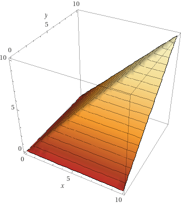
Here, there is no substitution between capital and labor and the production will be constrained by the minimum of the two production factors. Suppose the labor factor, x, is equal to five. In the contour plot, you will not observe an increase in production when you increase the capital factor beyond five, as you stay in the same reddish area above the point with the coordinates x = 5; y = 5. Production is not possible only one factor, as you can see in the reddest area of the graph for the points (x = 10; y = 0) and (y = 0; x = 10).

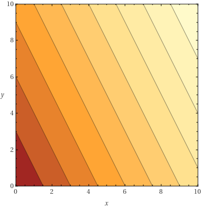
We continue with the linear production function. You have to go to the Wolfram Alpha website and enter one of the two formulas:

plot | f(x, y) = (2/3 x^1 + 1/3 y^1)^1 | x = 0 to 10 | y = 0 to 10

Plot3D[((2/3) x^1 + (1/3) y^1)^1, {x, 0, 10}, {y, 0, 10}]

This code will produce two figures, the first one is a 3D figure and the second one is a contour plot.

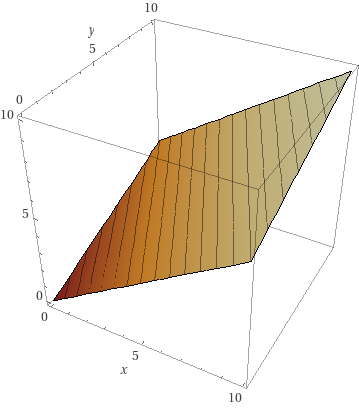
Here, there is substitution between capital and labor and we can always substitute capital and labor (and vice-versa) to produce. Suppose the labor factor, x, is equal to five. In the contour plot, you will observe an increase in production when you increase the capital factor beyond five, as you move to a yellowish area above the point with the coordinates x = 5; y = 5. Production is possible only one factor, as you can see in the points (x = 10; y = 0) and (y = 0; x = 10).

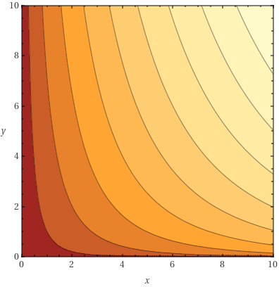
We conclude with the Cobb-Douglas production function. You have to go to the Wolfram Alpha website and enter one of the two formulas:

plot | f(x, y) = (2/3 x^0.1 + 1/3 y^0.1)^(1/0.1) | x = 0 to 10 | y = 0 to 10

Plot3D[((2/3) x^0.1 + (1/3) y^0.1)^(1/0.1), {x, 0, 10}, {y, -10., 10.}]

This code will produce two figures, the first one is a 3D figure and the second one is a contour plot.

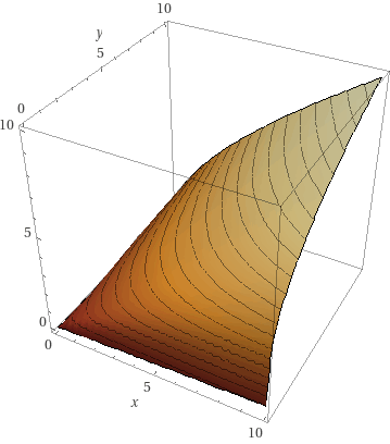
Here, there is substitution between capital and labor and we can substitute capital with a few labor if capital is high. Besides, we can substitute labor with a few capital if labor is high. Suppose the labor factor, x, is equal to five. In the contour plot, you will observe an increase in production when you increase the capital factor beyond five, as you move to more yellowish areas above the point with the coordinates x=5; y=5. Production is not possible only one factor, as you can see in the reddest area of the graph for the points (x = 10; y = 0) and (y = 0; x = 10).

Now, you can visualize by yourself and change the value of these production functions with some calibration about the labor and capital shares or switch to the case with increasing return of scale, for example.