Improving the visualization of time-varying coefficients

In this blog, I will show you how to improve the visualization of the time-varying coefficients of the estimator proposed by Inoue et al. (2024). I will leverage a previous blog of mine:

I will use the data and code coming from a previous research of mine written with Russell Smyth and Joaquin Vespignani:

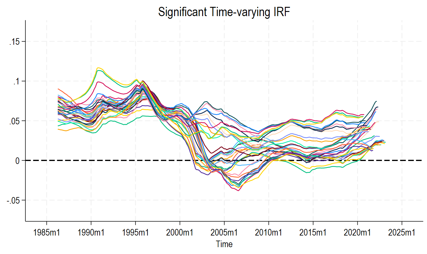
The graphs that I am going to produce:

The code below is annotated at each step:

**# Step 1: store the IRF estimates

// Summarize the observation to know the degree of freedom
summ LCu LGPRT GECON LGINF e1

// Display the post-estimation matrices
ereturn list

// Important informations
*number of lags = 12
*sample size for the shortest series = 473
*e(T) =  461 (473-12)
*e(q) =  63 (5 variables*12 lags + 1 constant + 1 y(t) + 1 shock)
*e(beta) :  3087 x 461

	
// Start the time-varying plots at the beginging of the sample
display tm(1985m1)
drop if period<=314 // After 12 lags for the shortest series

// Drop previous estimator paths and lower/upper bounds
cap drop a_* 
cap drop lb_* 
cap drop ub_*
cap drop airf_*
cap drop lbirf_*
cap drop ubirf_*

// Store the time-varying IRF estimates in a matrix and transpose it  
matrix list e(beta)
matrix tvlp_path=e(beta)'

// Put the time-varying IRF estimates in series
svmat double tvlp_path, name(a_) 

// Remove the abbrevation of the variables
set varabbrev off

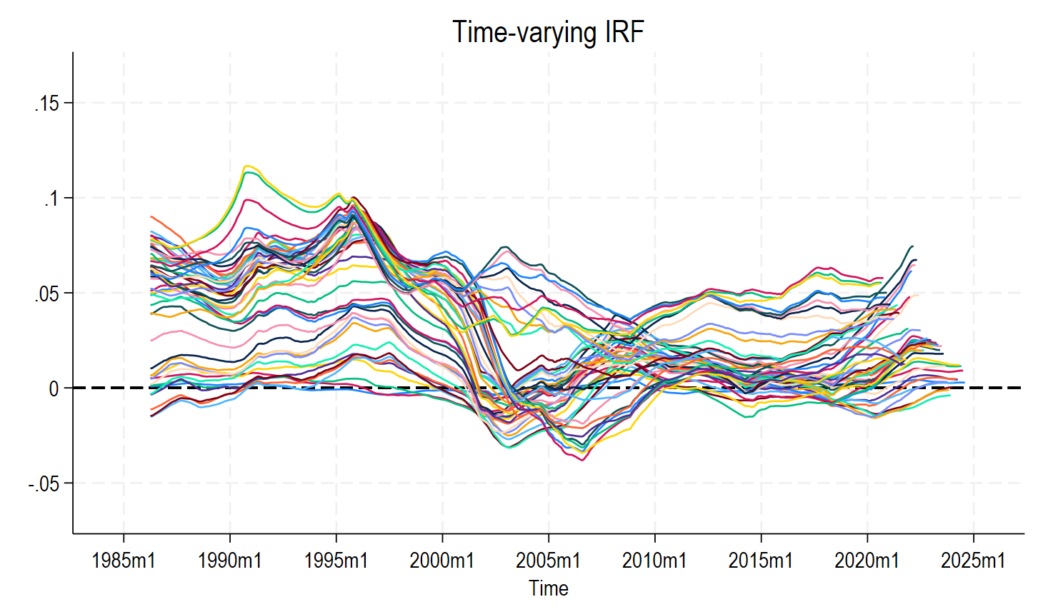
// Use a loop to plot time-varying IRF
set scheme stcolor
forvalues i = 1(63)3025 {
	local graphs `graphs' (tsline a_`i' if a_`i'!=0, legend(off) ///
	title("Time-varying IRF") xtitle("Time") yline(0) ///
	 plotregion(margin(large)))
	}	
graph twoway `graphs', name(TVplots, replace)

// Use a loop to keep the IRFs and drop the other series to save space
forvalues i = 1(63)3025 {
	rename a_`i' airf_`i', replace
	}
drop a_*

***************************************************************	

**# Step 2: store the lower bounds

// Store the time-varying IRFs' lower bounds in a matrix and transpose it  
matrix list e(beta_lb)
matrix tvlp_path_lb=e(beta_lb)'

// Put the time-varying IRF estimates in series
svmat double tvlp_path_lb, name(lb_) 

// Remove the abbrevation of the variables
set varabbrev off

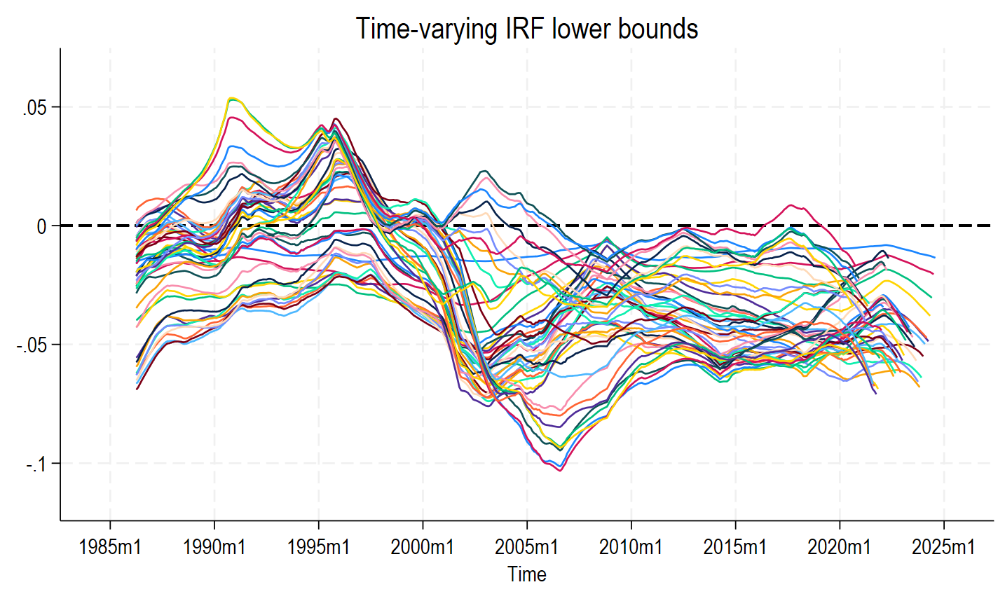
// Use a loop to plot time-varying IRF lower bounds
forvalues i = 1(63)3025 {
	local graphslb `graphslb' (tsline lb_`i' if lb_`i'!=0, legend(off) ///
	title("Time-varying IRF lower bounds") xtitle("Time") yline(0) ///
	 plotregion(margin(large)))
	}
graph twoway `graphslb', name(TVplots_lb, replace)

// Use a loop to keep the lower bounds and drop the other series to save space
forvalues i = 1(63)3025 {
	rename lb_`i' lbirf_`i', replace
	}
drop lb_*

***************************************************************	

**# Step 3: store the upper bounds

// Store the time-varying IRFs' upper bounds in a matrix and transpose it  
matrix list e(beta_ub)
matrix tvlp_path_ub=e(beta_ub)'

// Put the time-varying IRF estimates in series
svmat double tvlp_path_ub, name(ub_) 

// Remove the abbrevation of the variables
set varabbrev off

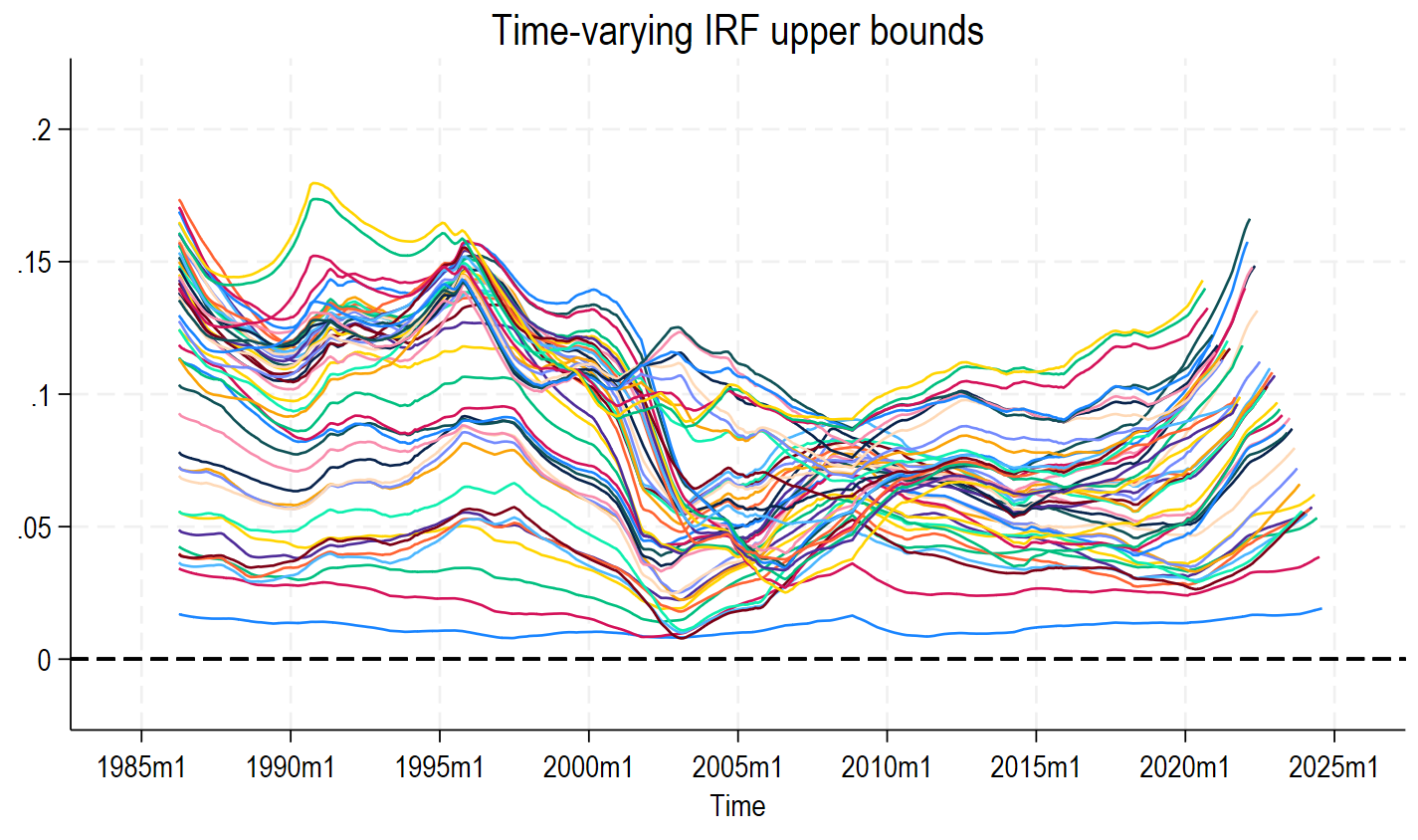
// Use a loop to plot time-varying IRF upper bounds
set scheme stcolor
forvalues i = 1(63)3025 {
	local graphsub `graphsub' (tsline ub_`i' if ub_`i'!=0, legend(off) ///
	title("Time-varying IRF upper bounds") xtitle("Time") yline(0) ///
	 plotregion(margin(large)))	
	}
graph twoway `graphsub', name(TVplots_ub, replace)

// Use a loop to keep the upper bounds and drop the other series to save space
forvalues i = 1(63)3025 {
	rename ub_`i' ubirf_`i', replace
	}
drop ub_*

***************************************************************	

// Use a loop to plot significant time-varying IRF
set scheme stcolor
forvalues i = 1(63)3025 {
	cap egen max_lbirf_`i' = max(lbirf_`i')
	local graphs `graphs' (tsline airf_`i' if max_lbirf_`i'>0 & ///
	airf_`i'!=0, legend(off) ///
	title("Significant Time-varying IRF") xtitle("Time") yline(0) ///
	 plotregion(margin(large)))
	}	
graph twoway `graphs', name(TVplotsA, replace)

***************************************************************

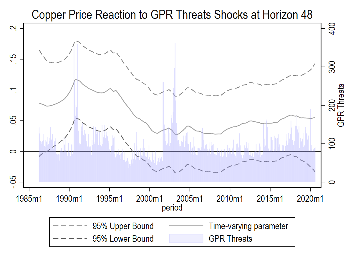
// Use the previous informations and change the scheme
*i = 1(63)3025
set scheme s1mono

// Start a counter that will help us to label the graphs
local x = 0 

// Start the loop for the graphs
forvalues i = 1(63)3025 {
	
lab var lbirf_`i' "95% Lower Bound"
lab var airf_`i' "Time-varying parameter"
lab var ubirf_`i' "95% Upper Bound"
lab var GPRT "GPR Threats"
	
twoway (tsline lbirf_`i' airf_`i' ubirf_`i' if airf_`i'!=0, ///
 yline(0) lpattern(dash solid dash)) ///
 bar GPRT period if airf_`i'!=0, yaxis(2) color(blue*0.4%20) ///
 title("Copper Price Reaction to GPR Threats Shocks at Horizon `x'") ///
 legend(order(3 "95% Upper Bound" ///
 2 "Time-varying parameter" 1 "95% Lower Bound" ///
 4 "GPR Threats")) ///
 name(TVplotsGPRT_`x', replace)
local ++x
}

// Save the graphs
forvalues i = 1(1)24 {	
 gr dis TVplotsGPRT_`i'
 gr export TVplotsGPRT_`i'.pdf, as(pdf) replace
 gr export TVplotsGPRT_`i'.png, as(png) replace
 }

Comments and remarks are welcome, as always!

References

Inoue, A., Rossi, B., & Wang, Y. (2024). Local projections in unstable environments. Journal of Econometrics, 105726.

Inoue, A., Rossi, B., & Wang, Y. (2024), ‘Has the Phillips Curve Flattened?‘ CEPR Discussion Paper No. 18846. CEPR Press, Paris & London. https://cepr.org/publications/dp18846

Saadaoui, J., Smyth, R., & Vespignani, J. (2025). Ensuring the security of the clean energy transition: Examining the impact of geopolitical risk on the price of critical minerals. Energy Economics, 142, 108195.