In this blog, I will show you how to visualize the time-varying coefficients of the estimator proposed by Inoue et al. (2024). The dataset used in this blog comes from a previous working paper of mine:
After running the tvpreg command, that will be released soon by the authors, you can display the stored result. To save space, I will use only six lags in the time-varying local projection (TV-LP) model. We obtain the following result. Please refer to the aforementioned working paper for more details:
// Blog (EconMacro)

ereturn list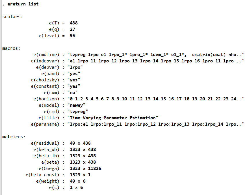
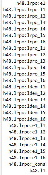
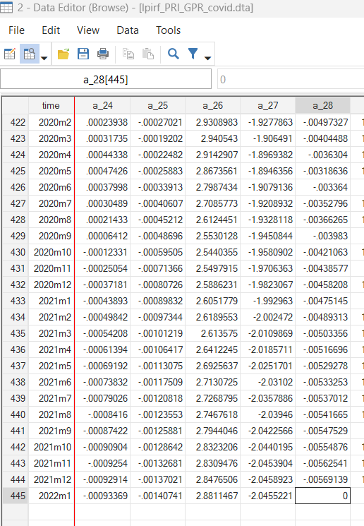
The sample size is equal to e(T) = 445-(6+1) and the number of time-varying parameters is given by e(q) = (4*6)+3. We have 49 horizons, from 0 to 48, as you can see in e(horizon). For the horizon 48, we have below the list of the time-varying parameters:
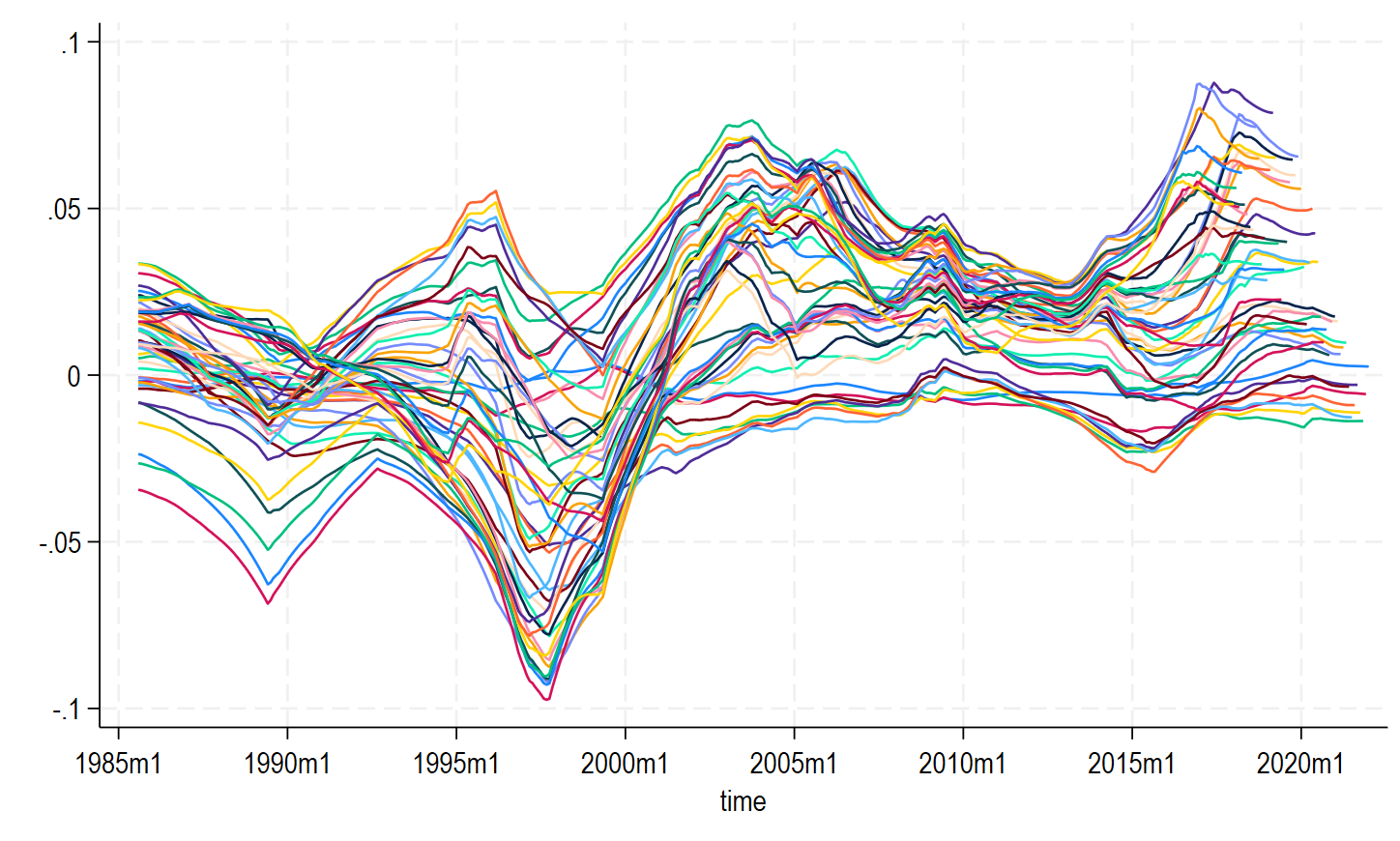
The next step consists in transforming the matrix e(beta) to series with the prefix a_:
matrix tvlp_path=e(beta)'
svmat double tvlp_path, name(a_)
set varabbrev off
set scheme stcolor
forvalues i = 1(27)1297 {
local graphs `graphs' (tsline a_`i' if a_`i'!=0, legend(off))
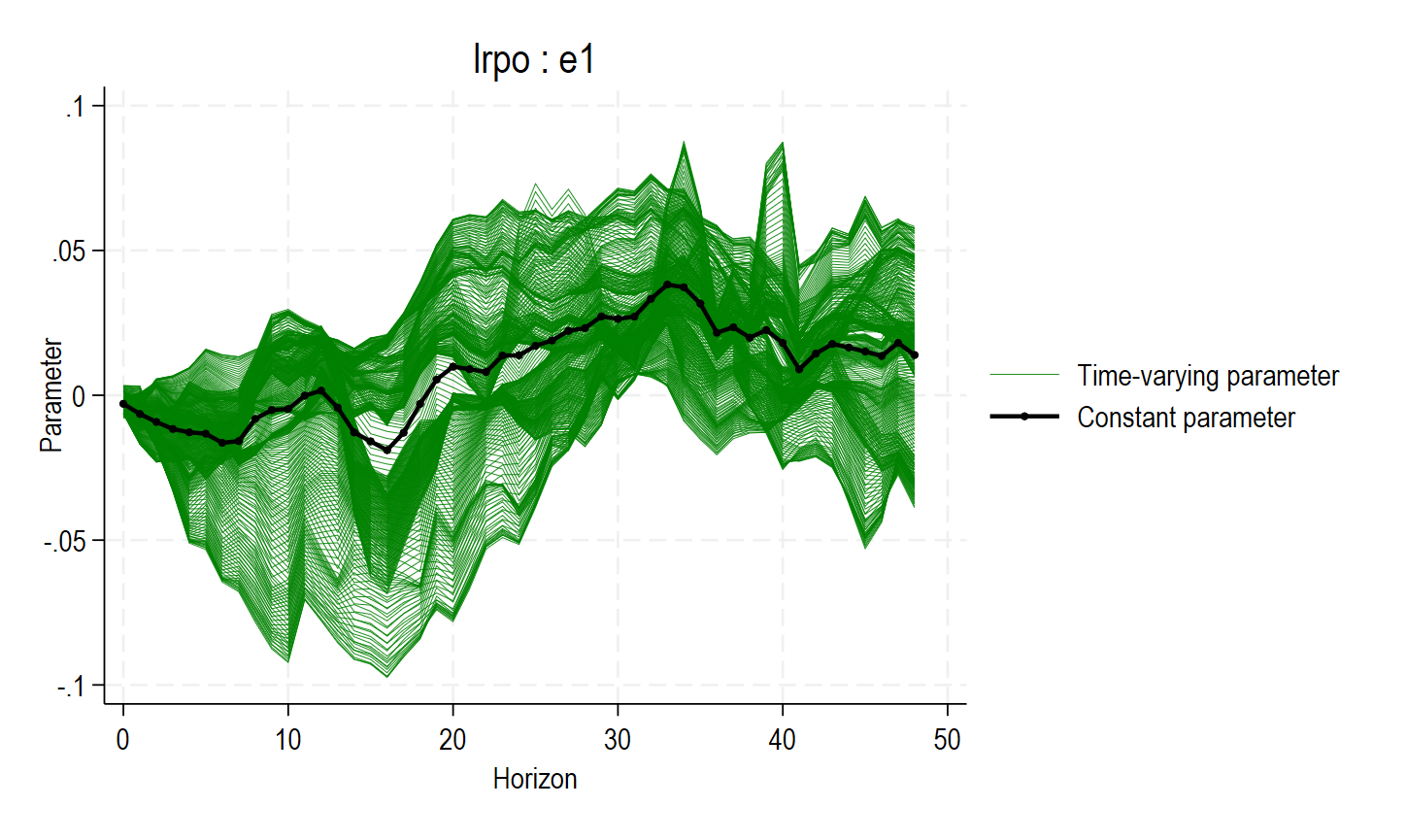
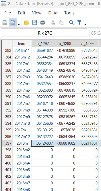
}As I am interested in the impact of the identified shock of geopolitical risk (e1) on the real price of oil in log (lrpo), I will select the first line of the matrix e(beta) at each horizon, so the loop will have the following number list: 1(27)1297. To obtain 1297, took the size of the matrix e(beta) and remove the number of time-varying parameters minus one (1323-(27-1)).
In the previous figure we plot the time-varying parameters for the IRFs at the different time horizons. For example, at the horizon 48, the sample starts in January 1985 and ends after T − h = 445 − 48 = 397 months in January 2018. Another example, at the horizon 1, the sample starts in January 1985 and ends after T − h = 445 − 1 = 444 months in December 2021.
The loop has been inspired by the following discussion on the Stata list. I thank David Radwin for this. I also thank Aikaterini Karadimitropoulou for pushing me to explore these graphs in more details.
Comments and remarks are welcome, as always!
References
Inoue, A., Rossi, B., & Wang, Y. (2024). Local projections in unstable environments. Journal of Econometrics, 105726.
Inoue, A., Rossi, B., & Wang, Y. (2024), ‘Has the Phillips Curve Flattened?‘ CEPR Discussion Paper No. 18846. CEPR Press, Paris & London. https://cepr.org/publications/dp18846
Saadaoui, J. (August 2024), The Impact of Political Tensions and Geopolitical Risks on Oil Prices in Unstable Environments. SSRN Working Paper 4921791.