In a few days, Alfonso Ugarte from BBVA will release an updated version of his package LOCPROJ. In this new version, the LPGRAPH command has been greatly improved and allows drawing the impulse response function with a few lines of codes.
You may be interested in looking at my series of blogs on LOCPROJ, I will use the data for the example used in the two last blogs. More information can be found in the following working paper: ADB Economics Working paper 748.
After these few words of introduction, let us start with the main topic of this blog. In this new version of LOCPROJ, you can visualize what is happening before the shock:
**# Negative horizon

locproj bonds_tw, shock(Dvul100) ///
 z h(-1/5) yl(1) sl(1) ///
 c(i.period) ///
 fe cluster(imfcode) conf(90 95) ///
 ttitle("Horizon") ///
 title(`"Impact of Change in Vulnerability on Bonds Yields"') ///
save irfname(vul_bonds) noisily 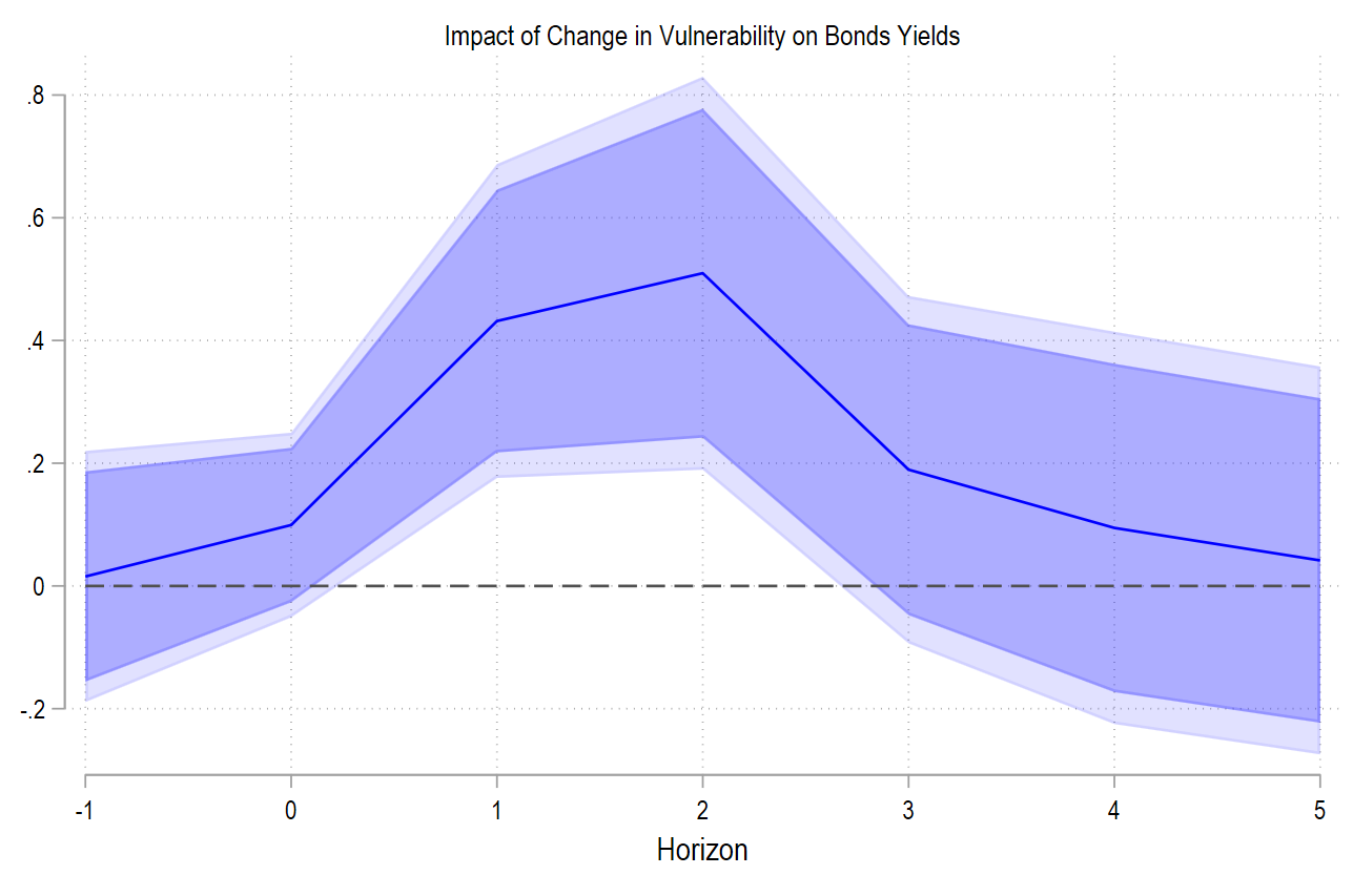
You can also plot different impulse response functions in a very convenient way. Here, I plot 95 percent confidence intervals and I include country and time fixed effects:
**# LP Graph

summ rel, detail

locproj bonds_tw if rel>5.625, shock(Dvul100) ///
 z h(4) yl(1) sl(1) ///
 c(i.period) ///
 fe cluster(imfcode) conf(95) ///
 ttitle("Horizon") ///
 title(`"Low Religious Tensions"') ///
 save irfname(vulhigh) noisily

locproj bonds_tw if rel<5.625, shock(Dvul100) ///
 z h(4) yl(1) sl(1) ///
 c(i.period) ///
 fe cluster(imfcode) conf(95) ///
 ttitle("Horizon") ///
 title(`"High Religious Tensions"') ///
 save irfname(vullow) noisily

lpgraph vulhigh vullow, ttitle("Horizon") h(4) ///
 title(`"Impact of Change in Vulnerability"') ///
 lab1(Low Religious Tensions) lab2(High Religious Tensions) ///
 ti1("Bonds Yields IRF - Levels") ///
 ti2("Bonds Yields IRF - Levels") ///
 lc1(red) lc2(blue) zero legend(pos(6)) ///
 grname(lpgraph) grsave(lpgraph) as(png)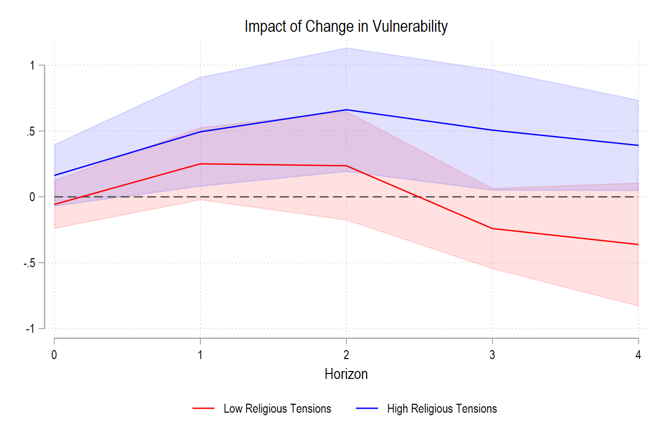
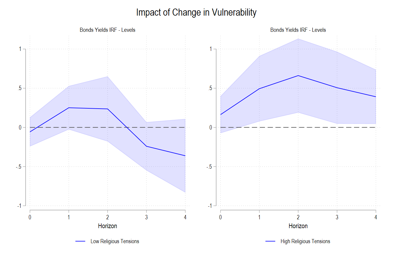
summ rel, detail

locproj bonds_tw if rel>5.625, shock(Dvul100) ///
 z h(4) yl(1) sl(1) ///
 c(i.period) ///
 fe cluster(imfcode) conf(95) ///
 ttitle("Horizon") ///
 title(`"Low Religious Tensions"') ///
 save irfname(vulhigh) noisily

locproj bonds_tw if rel<5.625, shock(Dvul100) ///
 z h(4) yl(1) sl(1) ///
 c(i.period) ///
 fe cluster(imfcode) conf(95) ///
 ttitle("Horizon") ///
 title(`"High Religious Tensions"') ///
 save irfname(vullow) noisily

lpgraph vulhigh vullow, ttitle("Horizon") h(4) ///
 title(`"Impact of Change in Vulnerability"') ///
 lab1(Low Religious Tensions) lab2(High Religious Tensions) ///
 ti1("Bonds Yields IRF - Levels") ///
 ti2("Bonds Yields IRF - Levels") ///
 lc1(red) lc2(blue) zero legend(pos(6)) ///
 grname(lpgraph) grsave(lpgraph) as(png) separate ///
 combine(ycommon)
With ‘grsave’ and ‘as’, you can save the graph in a very convenient way. If you want to have separate graphs, you can add the ‘separate’ option:
This command will be presented during my Timberlake training, which will take place on 19th February 2025 online:
https://www.timberlake.co.uk/courses/local-projections-25.html