In 10 days, I will present a recent research in the French/Japanese conference on Asian and International Economies in an Era of Globalization. In this research, we use time-varying causality tests. So today, I will show how to use the time-varying Granger causality tests introduced by Barbara Rossi and Yiru Wang in 2019:
Rossi, B., & Wang, Y. (2019). Vector autoregressive-based Granger causality test in the presence of instabilities. The Stata Journal, 19(4), 883-899.
We are going to replicate the results of Appendix in the following article:
Afonso, A., Mignon, V., & Saadaoui, J. (2024). On the time-varying impact of China’s bilateral political relations on its trading partners:“Doux commerce” or “trade follows the flag”? China Economic Review, 85, 102184.
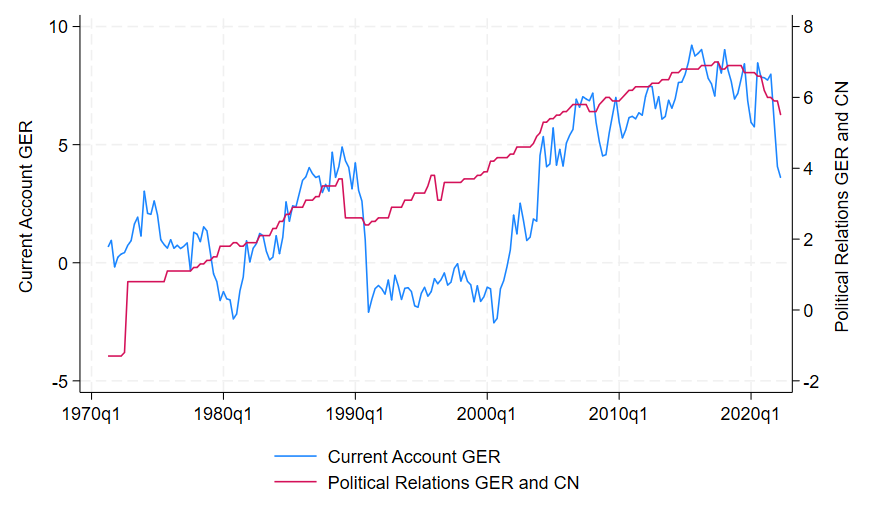
First things first, let us take a look at the two series:

The alternative approach proposed by Rossi and Wang (2019) to test Granger non-causality in the presence of instability in the case of the following two relationships (lpriger, is the index of political relationships between China and Germany; curger, is the current account balance of Germany; xrger, is the exchange rate, EUR/USD):
lpriger \xrightarrow{\mathrm{GC} ?} xrger

\\

lpriger \xrightarrow{\mathrm{GC} ?} cabger.
Small remark: As recommended by Andrew Sun, use the [ latex ]...[ /latex ] shortcode to insert an inline equation on WordPress if you are using the KaTeX plugin:
andrewsun.com/projects/wp-katex/
Firstly, their approach consists in using a reduced-form VAR with time-varying parameters,
\begin{aligned}
A_t(L) \mathbf{y}_t & =\mathbf{u}_t \quad \text{(A.1)}\\
A_t(L) & =\mathbf{I}-\mathbf{A}_{1, t} L-\cdots-\mathbf{A}_{p, t} L^p \\
\mathbf{u}_t & \stackrel{\text { i.i.d}}{\sim}(\mathbf{O}, \mathbf{\Sigma})
\end{aligned}
where \mathbf{y}_{t}=\left[y_{1, t}, y_{2, t}, \ldots, y_{n, t}\right]^{\prime} is an (n \times 1) vector and \mathbf{A}_{j, t}, j=1, \ldots, p, are (n \times n) time-varying coefficient matrices.
Secondly, they also consider a direct multistep VAR-LP (LP stands for Local Projection) forecasting with time-varying parameters. By iterating (A.1), \mathbf{y}_{t+h} can be projected onto the linear space generated by \left(\mathbf{y}_{t-1}, \mathbf{y}_{t-2}, \ldots, \mathbf{y}_{t-p}\right)^{\prime}, specifically,
\mathbf{y}_{t+h}=\boldsymbol{\Phi}_{1, t} \mathbf{y}_{t-1}+\cdots+\boldsymbol{\Phi}_{p, t} \mathbf{y}_{t-p}+\boldsymbol{\epsilon}_{t+h} \quad \text{(A.2)}where \boldsymbol{\Phi}_{j, t}, j=1, \ldots,p are functions of \mathbf{A}_{j, t}, \quad j=1, \ldots, p in (A.1) and \boldsymbol{\epsilon}_{t+h} is a moving average of the errors \mathbf{u} from time t to t+h in (A.1) and therefore uncorrelated with the regressors but serially correlated itself.
Let \boldsymbol{\theta}_t be an appropriate subset of \operatorname{vec}\left(\boldsymbol{\Phi}_{1, t}, \boldsymbol{\Phi}_{2, t}, \ldots, \boldsymbol{\Phi}_{p, t}\right). The null hypothesis of the Granger causality robust test is
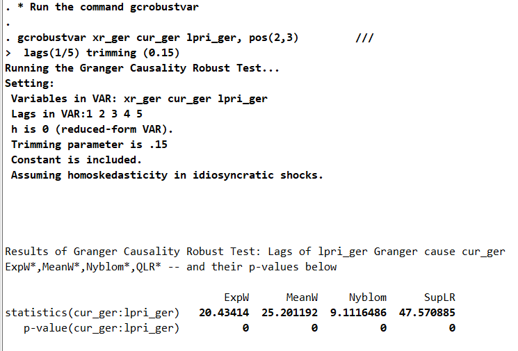
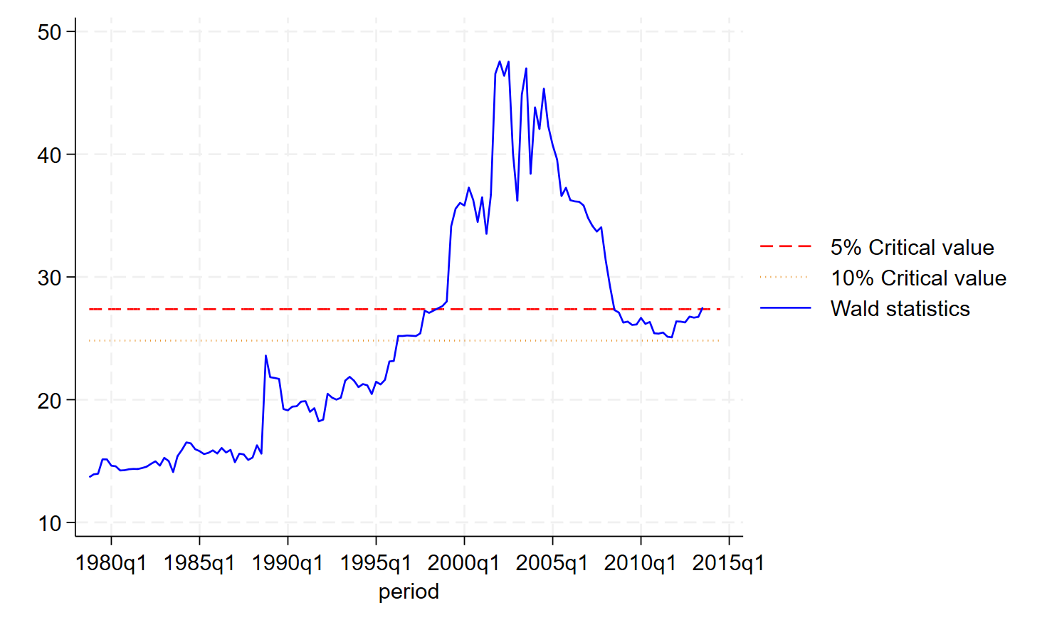
H_0: \boldsymbol{\theta}_t=\mathbf{0}\quad\forall t=1,2 \ldots T \quad \text{(A.3)}The statistics to test H0 in (A.3), presented in Rossi (2005), are ExpW* (the exponential Wald test), MeanW* (the mean Wald test), Nyblom* (the Nyblom test), and QLR* (the Quandt likelihood-ratio test).
The archive describes very well the file available for the replication, so I reproduce the read.me file below:
----------------------------------------------------------------------------
Guidance for implementation:
pvtable.mmat is the file storing pvalue tables;
gcrobustvar.ado is the command to run the VAR-based Granger-causality robust test. There are three commands used in gcrobustvar.ado: chowgmmstar3.ado, nyblomstar3.ado, pvcalc.ado.
Let us take a look at the full code, where each important step is commented:
*******************************************************

* Store the data in the same folder as the code and programs

use quaterly_dataset_all_wald_17aug2023.dta, clear

*Drop missing variables

drop if period<tq(1971q1)
drop if period>tq(2022q2)

** Drop the starting value to not have missing values

drop if period<tq(1971q2)

gen trend=_n

****************************************************************

twoway line cur_ger period if period>=00, yaxis(1) || ///
 line pri_ger_cn period if period>=00, yaxis(2) ///
 legend(pos(6)) xtitle("") ///
 name(cur_pri_china_ger, replace)

* Install package

/*
net from http://www.stata-journal.com/software/sj19-4/
net describe st0581
net install st0581, force
net get st0581, force
*/

* Load the critical values

mata:
mata clear
mata matuse pvtable, replace
st_matrix("r(pvap0opt)",pvap0opt)
st_matrix("r(pvapiopt)",pvapiopt)
st_matrix("r(pvnybopt)",pvnybopt)
st_matrix("r(pvqlropt)",pvqlropt)
end

matrix pvap0opt=r(pvap0opt)
matrix pvapiopt=r(pvapiopt)
matrix pvnybopt=r(pvnybopt)
matrix pvqlropt=r(pvqlropt)

* Don't forget to install matsqrt

/*
quietly ///
net describe matsqrt, from(http://www.stata.com/users/jpitblado)
quietly net install matsqrt
*/

* Run the command gcrobustvar

gcrobustvar xr_ger cur_ger lpri_ger, pos(2,3) ///
 lags(1/5) trimming (0.15)
graph rename Graph lpri_ger_cur_ger, replace

* Export the figure

graph export lpri_ger_cur_ger_blog.png, replace ///
 name(lpri_ger_cur_ger)
graph export lpri_ger_cur_ger_blog.pdf, replace ///
 name(lpri_ger_cur_ger)

*******************************************************

If you want to run the command a second time, you may have to create a Do-file, that I called gc_robust.do:
*Store the data in the same folder as the code and programs

use quaterly_dataset_all_wald_17aug2023.dta, clear

*Drop missing variables

drop if period<tq(1971q1)
drop if period>tq(2022q2)

** Drop the starting value to not have missing values

drop if period<tq(1971q2)

gen trend=_n

mata:
mata clear
mata matuse pvtable, replace
st_matrix("r(pvap0opt)",pvap0opt)
st_matrix("r(pvapiopt)",pvapiopt)
st_matrix("r(pvnybopt)",pvnybopt)
st_matrix("r(pvqlropt)",pvqlropt)
end

matrix pvap0opt=r(pvap0opt)
matrix pvapiopt=r(pvapiopt)
matrix pvnybopt=r(pvnybopt)
matrix pvqlropt=r(pvqlropt)
Then, I run a second time the command for the VAR-LP:
* VAR-LP

quietly do gcrobust_blog.do
/*
Run this to not have the error message:
variable time_chowgmmstar not found
 */

gcrobustvar xr_ger cur_ger lpri_ger, pos(2,3)         ///
 lags(1/5) trimming (0.15) horizon(5)
graph rename Graph lpri_ger_cur_ger, replace
After the mid-1990s, we reject the null of non-causality. The trade always follows the flag between Germany and China. Montesquieu may be wrong:
4 Comments
I am still getting the error: variable time_chowgmmstar not found
See the last part of the blog:
“If you want to run the command a second time, you may have to create a Do-file, that I called gc_robust.do:”
Thank you very much Proff, it worked. I have been struggling for days.
You’re welcome Jason.
Please don’t hesitate to ask something else.