State-Dependent Local Projections using LOCPROJ

A few days ago, I read the Country Risk Annual Report made by BBVA research and Alfonso Ugarte and David Sarasa Flores, in particular.

On the slide 26, they estimate the dynamic impact of rules compliance on sovereign bond spreads by the following panel state-dependent local projection regressions (Ramey and Zubairy (2018)), conditioned on the level of debt-to-GDP (below or above 90%) using the Stata package LOCPROJ, written by Alfonso Ugarte.

In my previous research, I relied on subsample analyses to capture this “state dependence” of the impact of climate risk shocks on government bonds conditional on the level of religious tensions.

Splitting the sample between high and low religious tensions produces the following results:

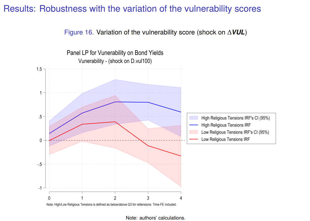
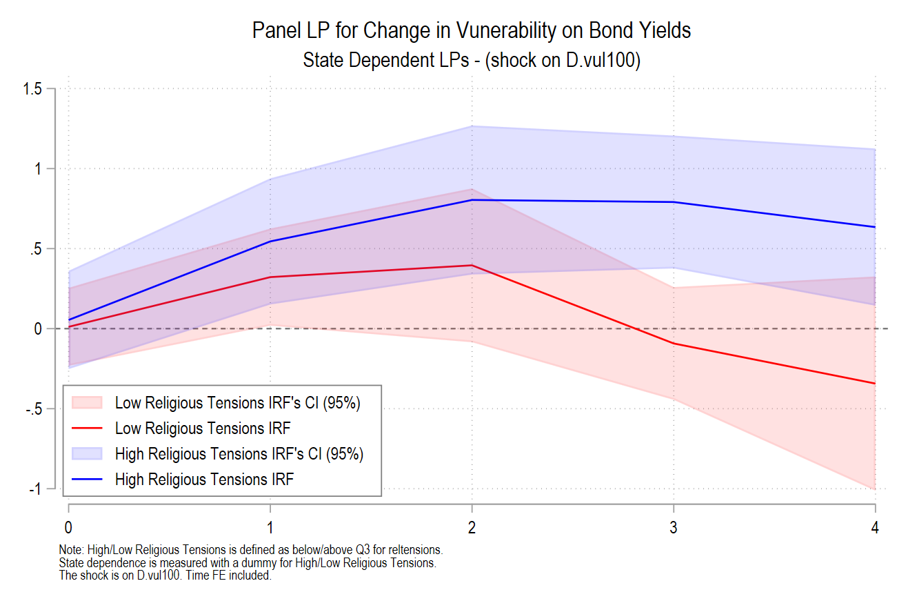
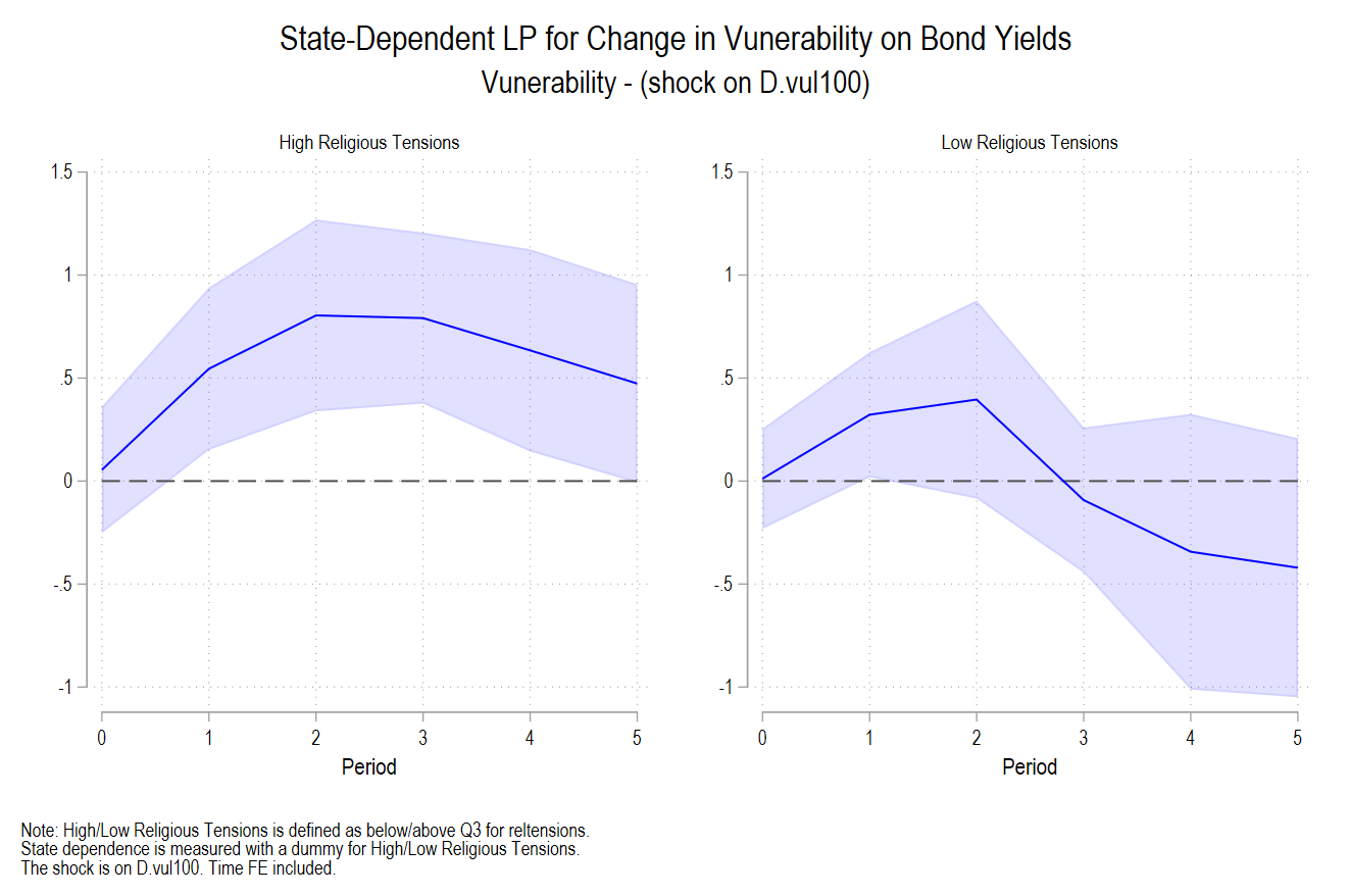
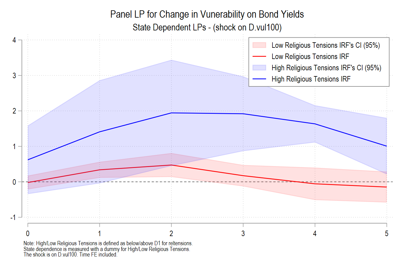
More details are available about this original result in the literature on the climate risk premium in this ADB working paper. One advantage of using a state-dependent panel LP approach will be to not rely on subsample and preserve the sample size. This can be formulated in the following way, when the risk rating of religious is low, that means the risk of the religious tension is high:

\small
\begin{equation*}
\begin{split}

\textit{bonds}_{i, t+h}  = \alpha_i^h+ \gamma_1 \cdot \textit{bonds}_{i, t-1} \thickspace\thickspace\thickspace\thickspace\thickspace\thickspace\thickspace\thickspace\thickspace\thickspace\thickspace\thickspace\thickspace\thickspace\thickspace\thickspace\thickspace\thickspace\thickspace\thickspace\\

+\mathbf{1}\left[rel_{i,t-1}>relQ3_{i,t-1}\right]\left(\beta_{low}^h \Delta VUL_{i, t-1}\right) \\   

+ \mathbf{1}\left[rel_{i, t-1} \leq relQ3_{i,t-1}\right]\left(\beta_{high}^h \Delta VUL_{i, t-1}\right) \\

+\mathbf{X}_{i, t-1} \delta^h+\epsilon_{i, t}^h

\end{split}
\end{equation*}

Following the advice of Alfonso Ugarte, I propose the following code:

**#* State-dependent LPs

**#* Religious Tensions

// Bonds - High Religious Tensions

sum reltensions, detail

egen reltensions_p75 = pctile(reltensions), p(75)

cap drop D
gen D = 0
replace D = 1 if reltensions<reltensions_p75

locproj bonds_tw D#c.Dvul100, lcs(1.D#c.Dvul100) ///
 h(5) yl(1) sl(1) ///
 c(l(1).CAB l(1).cpi_tw l(1).GDebt l(1).GDeficit ///
   l(1).bondsUS_tw ///
   l(1).msciworld_gw l(1).VIXCLS ///
   l(1).banking l(1).currency l(1).debt i.period) ///
 fe cluster(imfcode) conf(95) ///
 save irfname(below)
 graph rename Graph below, replace
 
locproj bonds_tw D#c.Dvul100, lcs(0.D#c.Dvul100) ///
 h(5) yl(1) sl(1) ///
 c(l(1).CAB l(1).cpi_tw l(1).GDebt l(1).GDeficit ///
   l(1).bondsUS_tw ///
   l(1).msciworld_gw l(1).VIXCLS ///
   l(1).banking l(1).currency l(1).debt i.period) ///
 fe cluster(imfcode) conf(95) ///
 save irfname(high)
graph rename Graph high, replace

cap by imfcode: gen N = _n-1

twoway ///
 (rarea high_up high_lo N, fcolor(red%15) ///
  lc(red%7)) ///
 (line high N, lcolor(red) lpattern(solid)) ///
 (rarea below_up below_lo N, ///
  fcolor(blue%15) lc(blue%7)) ///
 (line below N, lcolor(blue) lpattern(solid)) ///
  if N<5, xtitle("")  yline(0) ///
 title(`"Panel LP for Change in Vunerability on Bond Yields"') ///
 subtitle(`"State Dependent LPs - (shock on D.vul100)"') ///
 legend(pos(7) ring(0) size(small) ///
 label(1 "Low Religious Tensions IRF's CI (95%)") ///
 label(2 "Low Religious Tensions IRF") ///
 label(3 "High Religious Tensions IRF's CI (95%)") ///
 label(4 "High Religious Tensions IRF") ///
 region(lcolor(gray))) name(bonds_reltensions, replace) ///
 note("Note: High/Low Religious Tensions is defined as below/above Q3 for reltensions." "State dependence is measured with a dummy for High/Low Religious Tensions." "The shock is on D.vul100. Time FE included.", size(vsmall))
 
graph export SD_LPs_reltensions_dec24.png, as(png) width(4000) replace

These empirical results are very similar to those relying on subsamples:

This joint work is written with John Beirne, Donghyun Park and Gazi Salah Uddin: ADB Economics Working paper 748.

Our causal identification relies on the fact that government bond yields and sovereign ratings on foreign currency debt do not influence changes in the ND-GAIN vulnerability scores at any horizon.

Key results:
▶️ Political stability reduces the fiscal impact of climate vulnerability risks
▶️ Financial development also limits the climate risk premium
▶️ The most vulnerable economies face the largest climate-related fiscal risks
▶️ Religious tensions are the most impactful form of political instability (State-dependence confirms subsample analyses)
▶️ Stable politics and strong markets together mitigate fiscal risks