Drawing maps at different regional levels

1 Introduction

This short note aims to demonstrate the drawing of choropleth maps at different regional levels thanks to Natural Earth Data and GADM data. Drawing maps on Stata may be perceived as complex by some practitioners and, particularly, by students. In the following, I will show you the main principles that can be used to draw some detailed and customized maps at different regional levels.

2 Natural Earth Data

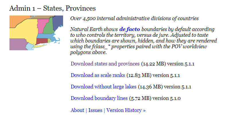
The first step will consist in downloading the files to build the map on the following website: https://www.naturalearthdata.com/downloads/10m-cultural-vectors/. In the download tab, I choose the 1:10m Cultural Vectors and the Admin 1 – States, Provinces level. The .dbf and .shp files have to be unzipped and put into the folder that will contain the data. The spshape2dta package will build the files necessary to draw the maps.

graph set window fontface "Palatino Linotype"

unzipfile "ne_10m_admin_1_states_provinces.zip", replace

**# **** Maps with Natural Earth data for China ****************

spshape2dta ne_10m_admin_1_states_provinces, replace

Thanks to the .dbf and .shp files, spshape2dta package will produce two files .dta with important information, as you can read in the two last lines in the following. The first one will contain the coordinates and the second one will contain the names of the regions. I use the second file where the ID, the coordinates (longitude and latitude) are included among with other information like the name of the regions and other useful information like the other sovereignty or the Wiki Data ID.

. spshape2dta ne_10m_admin_1_states_provinces, replace
  (importing .shp file)
  (importing .dbf file)
  (creating _ID spatial-unit id)
  (creating _CX coordinate)
  (creating _CY coordinate)
  
  file ne_10m_admin_1_states_provinces_shp.dta created
  file ne_10m_admin_1_states_provinces.dta created
.

Then, I will generate a variable that is equal to the number of characters in the name of the administrative division for China in Figure 1, thanks to the ISO A2 code, and export it in PNG and PDF format. To produce Figure 2, I just need to change the option label(name) to label(name_zht).

**#*** Draw the map for Chinese regions ************************

use ne_10m_admin_1_states_provinces.dta, clear 

// Run everything between preserve and restore

grmap, activate

generate length = strlen(name)

preserve

keep if iso_a2 == "CN" & name != "Paracel Islands"

grmap length using ne_10m_admin_1_states_provinces_shp.dta, ///
 fcolor(Blues) ///
 osize(vvthin ..) ///
 ndsize(vvthin) ///
 ndfcolor(gray) clmethod(quantile) ///
 title("Region name length") label(xcoord(_CX) ycoord(_CY) ///
 label(name) size(*.5))
 
graph rename Graph map_china_regions, replace

graph export map_china_regions.png, as(png) ///
 width(4000) replace
graph export map_china_regions.pdf, as(pdf) ///
 replace

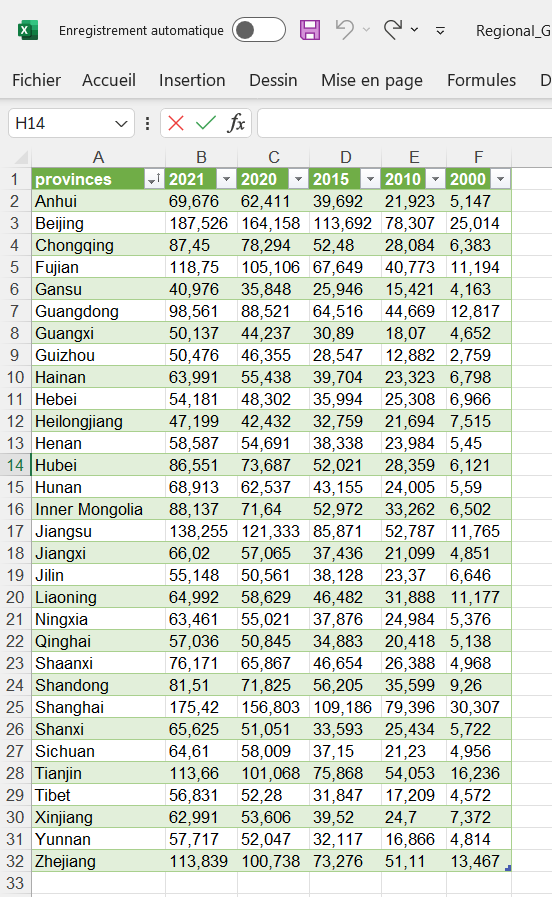
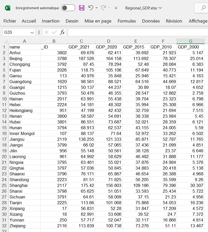
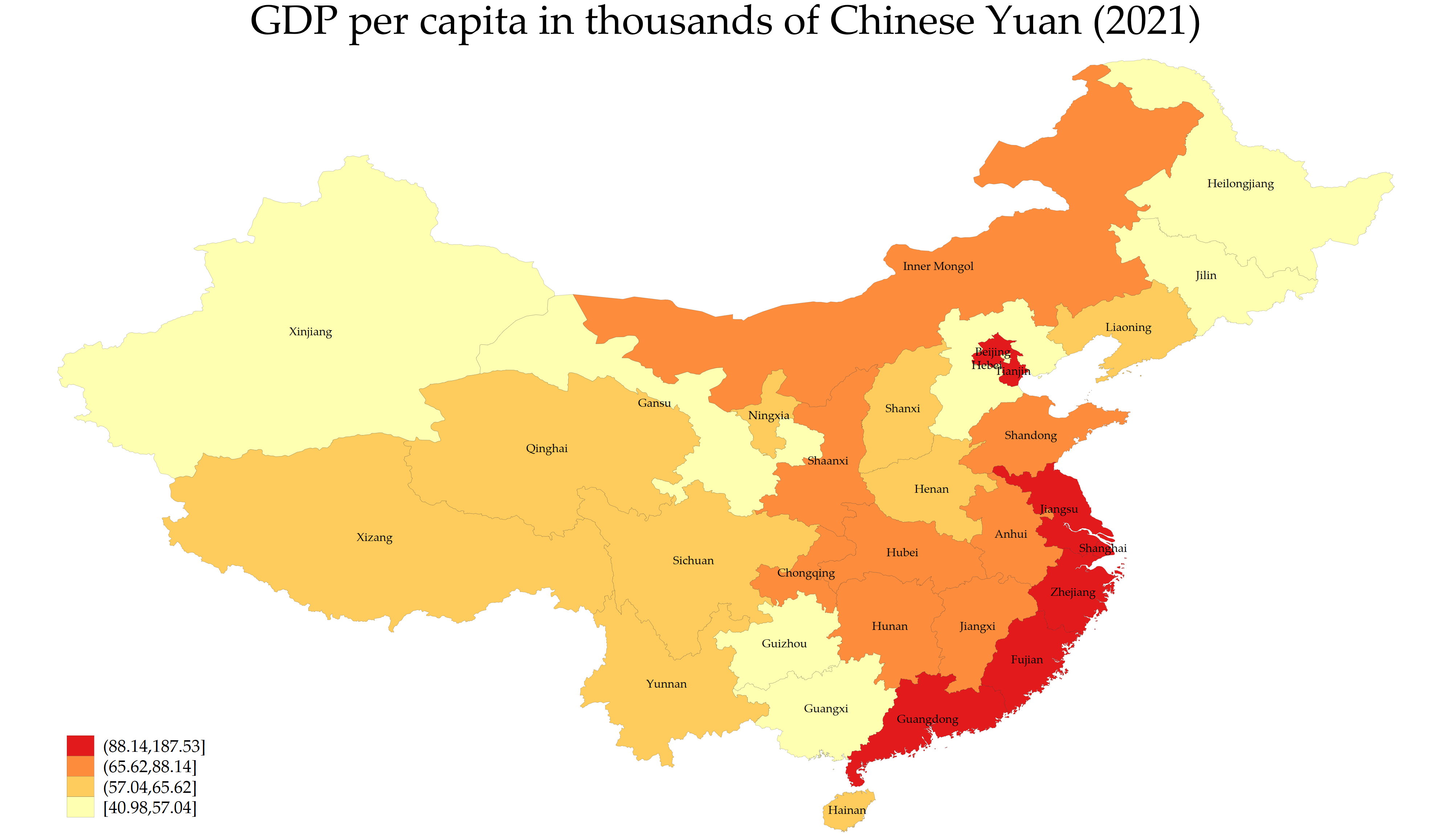
restore

Finally, I can add some data for the Chinese regional GDP and merge them with the regional GDP of Chinese regions in Thousand of Yuan per capita (www.stats.gov.cn) thanks to the ID of the regions in Figure 3. The disparities between inner and coastal China are obvious. The data in the Excel file ’Regional GDP.xlsx’ for the regional GDP. I imported the data from Wikipedia in Excel, and especially, the table under the following title: ’GDP per capita in 31 provinces of mainland China by Chinese yuan (renminbi)’. In Excel, I use
’Data’ and ’Import from web’ with this URL. Finally, I create a new table for 31 Chinese provinces, where I add manually the corresponding _IDs (from the file ne_10m_admin_1_states provinces.dta) in a new Excel sheet called ’Feuil1’.

**#*** Draw the map for Chinese regional GDP *******************

// Download Regional GDP for China and merge it

import excel Regional_GDP.xlsx, sheet("Feuil1") ///
 cellrange(B1:G32) firstrow clear

save Regional_GDP.dta, replace 

use ne_10m_admin_1_states_provinces.dta, replace

// Merging regional GDP and IDs
merge 1:1 _ID using "Regional_GDP.dta", nogenerate

// Run everything between preserve and restore

preserve

format GDP_* %4.2f

keep if iso_a2 == "CN" & name != "Paracel Islands"

grmap GDP_2021 using ///
 ne_10m_admin_1_states_provinces_shp.dta, ///
 fcolor(YlOrRd)  ///
 osize(vvthin ..) ///
 ndsize(vvthin) ///
 ndfcolor(gray) clmethod(quantile) ///
 title("GDP per capita in thousands of Chinese Yuan (2021)") ///
 label(xcoord(_CX) ycoord(_CY) ///
 label(name) size(*.5) length(50))
 
graph rename Graph map_china_regions_gdp, replace

graph export map_china_regions_gdp.png, as(png) ///
 width(4000) replace
graph export map_china_regions_gdp.pdf, as(pdf) ///
 replace
 
restore

save maps_china_ne.dta, replace 
 
**#**** End of the program *************************************

Figure 1: Map of Chinese regions’ name length

Figure 2: Map of Chinese regions’ name length in Chinese

In the following, you can remark that the total number of ’regions’ (first administrative level) is equal to 4596 for more than 240 countries in the .dta file produced by the spshape2dta package:

// Merging regional GDP and IDs
merge 1:1 _ID using "Regional_GDP.dta", nogenerate
.
  Result Number of obs
  -----------------------------------------
  Not matched 4,565
  from master 4,565
  from using 0
  Matched 31
  ----------------------------------------
.

Figure 3: Map of Chinese regions’ GDP per capita in 2021

3 GADM Data

Now, I will use the Global Administrative Areas (GADM data to draw maps at four different administrative levels, thanks to data on the GADM website: https://gadm.org).

The data can be found on this GADM webpage: https://gadm.org/data.html. Then, choose the desired country and Shapefile. Let us start with the first administrative level in Austria. As explained in the previous section, I need to download the ZIP file containing the .dbf and .shp files. On the aforementioned page, select Austria and then pick the shapefile. Figure 4 displays the result for the region of Wien and Burgenland. Different regions can be selected by changing the IDs in the following option, select(keep if inlist(_ID,1,9)). The regions labels can be selected using different IDs in this option, label(xcoord(_CX) ycoord(_CY) select(keep if inlist(_ID,1,2,7,9)).

unzipfile "gadm41_AUT_shp.zip", replace

**# **** Maps with GADM data for Austria (Level 1) *************

spshape2dta gadm41_AUT_1, ///
 saving(gadm41_AUT_1) replace

use gadm41_AUT_1.dta, clear

generate length = strlen(NAME_1)

grmap length using gadm41_AUT_1_shp.dta, ///
	fcolor(Blues) ///
	ndfcolor(gray) clmethod(quantile) ///
	polygon(data(gadm41_AUT_1_shp.dta) ///
	select(keep if inlist(_ID,1,9)) ///
	fc(red) os(vvthin)) ///
	os(vvthin ..) ndsize(vvthin) ///
	title("Region name length [length]") ///
	label(xcoord(_CX) ycoord(_CY) ///
	select(keep if inlist(_ID,1,2,7,9)) ///
	label(NAME_1) size(5) length(22) pos(11) angle(340) ///
	gap(-3)) ///
	legend(pos(11) size(5)) legcount

graph rename Graph map_austria_1, replace
graph export map_austria_1.png, as(png) ///
 width(4000) replace
graph export map_austria_1.pdf, as(pdf) ///
 replace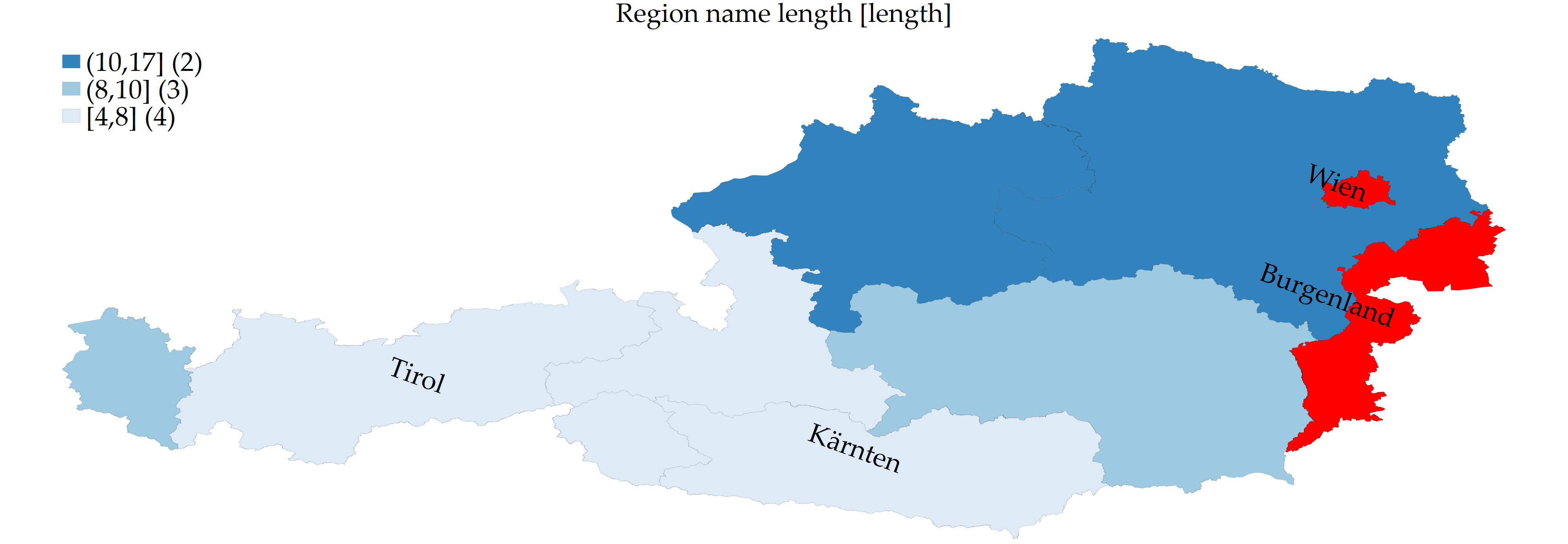

Figure 4: Map of Austria regions’ name length – Level 1

In the following Figures 5 to 7, I repeat the same process for the following administrative levels in Austria, namely, District, Municipality, Cadastral community. Finally, I zoom into the Wien Stadt region and highlight some Cadastral communities. I highlight and name some administrative entities following the help of the grmap package. The code for the Municipality level is very similar. I just changed it to use the second administrative level in Figure 5.

**# **** Maps with GADM data for Austria (Level 2) *************

spshape2dta gadm41_AUT_2, ///
 saving(gadm41_AUT_2) replace

use gadm41_AUT_2.dta, clear

generate length = strlen(NAME_2)

grmap length using gadm41_AUT_2_shp.dta, ///
	fcolor(Blues) ///
	ndfcolor(gray) clmethod(quantile) ///
	polygon(data(gadm41_AUT_2_shp.dta) ///
	select(keep if inlist(_ID,2,94)) ///
	fc(red) os(vvthin)) ///
	os(vvthin ..) ndsize(vvthin) ///
	title("Region name length [length]") ///
	label(xcoord(_CX) ycoord(_CY) ///
	select(keep if inlist(_ID,2,83,94)) ///
	label(NAME_2) size(5) length(22) pos(11) angle(340) ///
	gap(-3)) ///
	legend(pos(11) size(5)) legcount
 
graph rename Graph map_austria_2, replace
graph export map_austria_2.png, as(png) ///
 width(4000) replace
graph export map_austria_2.pdf, as(pdf) ///
 replace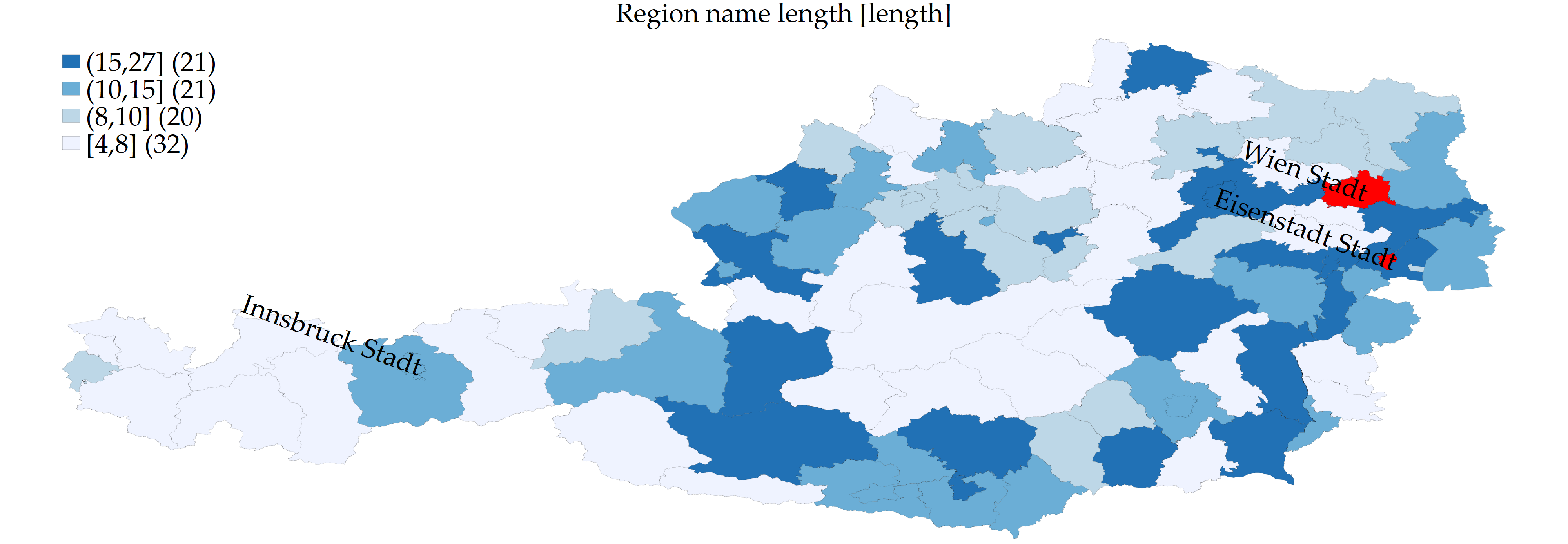

Figure 5: Map of Austria regions’ name length – Level 2

The codes for the two following examples (Levels 3 and 4 in Figure 6 and 7) are very similar and be available in the replication archive of this note.

**# **** Maps with GADM data for Austria (Level 3) *************
 
spshape2dta gadm41_AUT_3, ///
 saving(gadm41_AUT_3) replace

use gadm41_AUT_3.dta, clear

generate length = strlen(NAME_3)

grmap length using gadm41_AUT_3_shp.dta, id(_ID) ///
 fcolor(Reds)  ///
 ndfcolor(gray) clmethod(quantile) ///
  polygon(data(gadm41_AUT_3_shp.dta) ///
   select(keep if _ID==24 | ///
  _ID==2100 | _ID==1814) fc(yellow) os(vvthin)) ///
 os(vvthin vvthin vvthin vvthin) ndsize(vvthin) ///
 title("Region name length [length]") ///
 label(xcoord(_CX) ycoord(_CY) select(keep if _ID==24 | ///
  _ID==2100 | _ID==1814) ///
 label(NAME_3) size(5) length(22) pos(11) angle(340) ///
  gap(-3)) ///
 legend(pos(11) size(5)) legcount 
 
graph rename Graph map_austria_3, replace
graph export map_austria_3.png, as(png) ///
 width(4000) replace
graph export map_austria_3.pdf, as(pdf) ///
 replace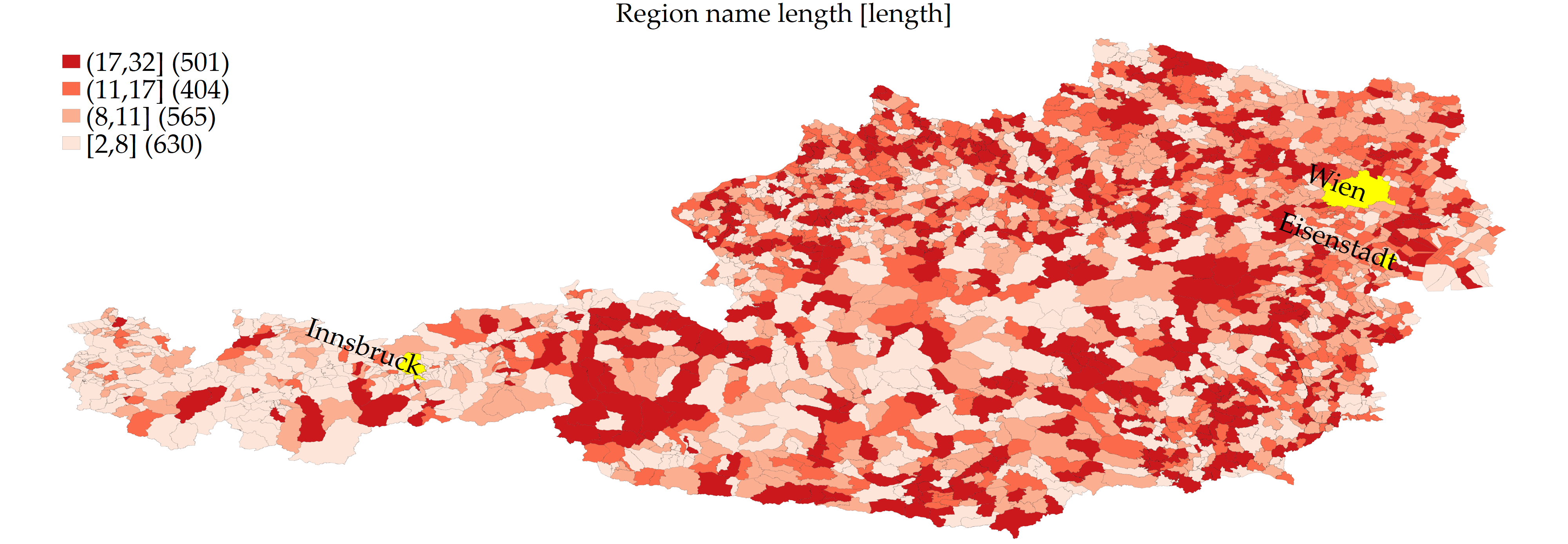

Figure 6: Map of Austria regions’ name length – Level 3

**# **** Maps with GADM data for Austria (Level 4) *************
 
spshape2dta gadm41_AUT_4, ///
 saving(gadm41_AUT_4) replace

use gadm41_AUT_4.dta, clear

generate length = strlen(NAME_4)

grmap length using gadm41_AUT_4_shp.dta, id(_ID) ///
 fcolor(Blues)  ///
 ndfcolor(gray) clmethod(quantile) ///
  polygon(data(gadm41_AUT_4_shp.dta) select(keep if ///
  _ID==7810 | _ID==25 | _ID==7406) fc(red) os(vvthin)) ///
 os(vvthin vvthin vvthin vvthin) ndsize(vvthin) //////
 title("Region name length [length]") ///
 label(xcoord(_CX) ycoord(_CY) select(keep if _ID==7810 | ///
  _ID==7810 | _ID==25 | _ID==7406) ///
  label(NAME_4) size(5) length(13) pos(8) angle(340) ///
  gap(0) color(black)) ///
 legend(pos(11) size(5)) legcount 
 
graph rename Graph map_austria_4, replace
graph export map_austria_4.png, as(png) ///
 width(4000) replace
graph export map_austria_4.pdf, as(pdf) ///
 replace

Figure 7: Map of Austria regions’ name length – Level 4

Finally, I make a Zoom a specific region, Wien Stadt, in Figure 8.

**# **** Maps with GADM data for Austria (Level 4 Zoom) ********

spshape2dta gadm41_AUT_4, ///
 saving(gadm41_AUT_4) replace

use gadm41_AUT_4.dta, clear

generate length = strlen(NAME_4)

grmap length using gadm41_AUT_4_shp.dta if _ID>=7762, ///
 fcolor(Blues) ///
 ndfcolor(gray) clmethod(quantile) ///
 polygon(data(gadm41_AUT_4_shp.dta) ///
 select(keep if inlist(_ID,7791,7810)) ///
 fc(red) os(vvthin)) ///
 os(vvthin ..) ndsize(vvthin) ///
 title("Region name length [length]") ///
 label(xcoord(_CX) ycoord(_CY) ///
 select(keep if inlist(_ID,7791,7810)) ///
 label(NAME_4) size(5) length(13) pos(8) angle(340) ///
 gap(0) color(black)) ///
 legend(pos(11) size(5)) legcount 

graph rename Graph map_austria_4bis, replace
graph export map_austria_4bis.png, as(png) ///
 width(8000) replace
graph export map_austria_4bis.pdf, as(pdf) ///
 replace
 
save maps_austria_gadm.dta, replace 
 
**#**** End of the program *************************************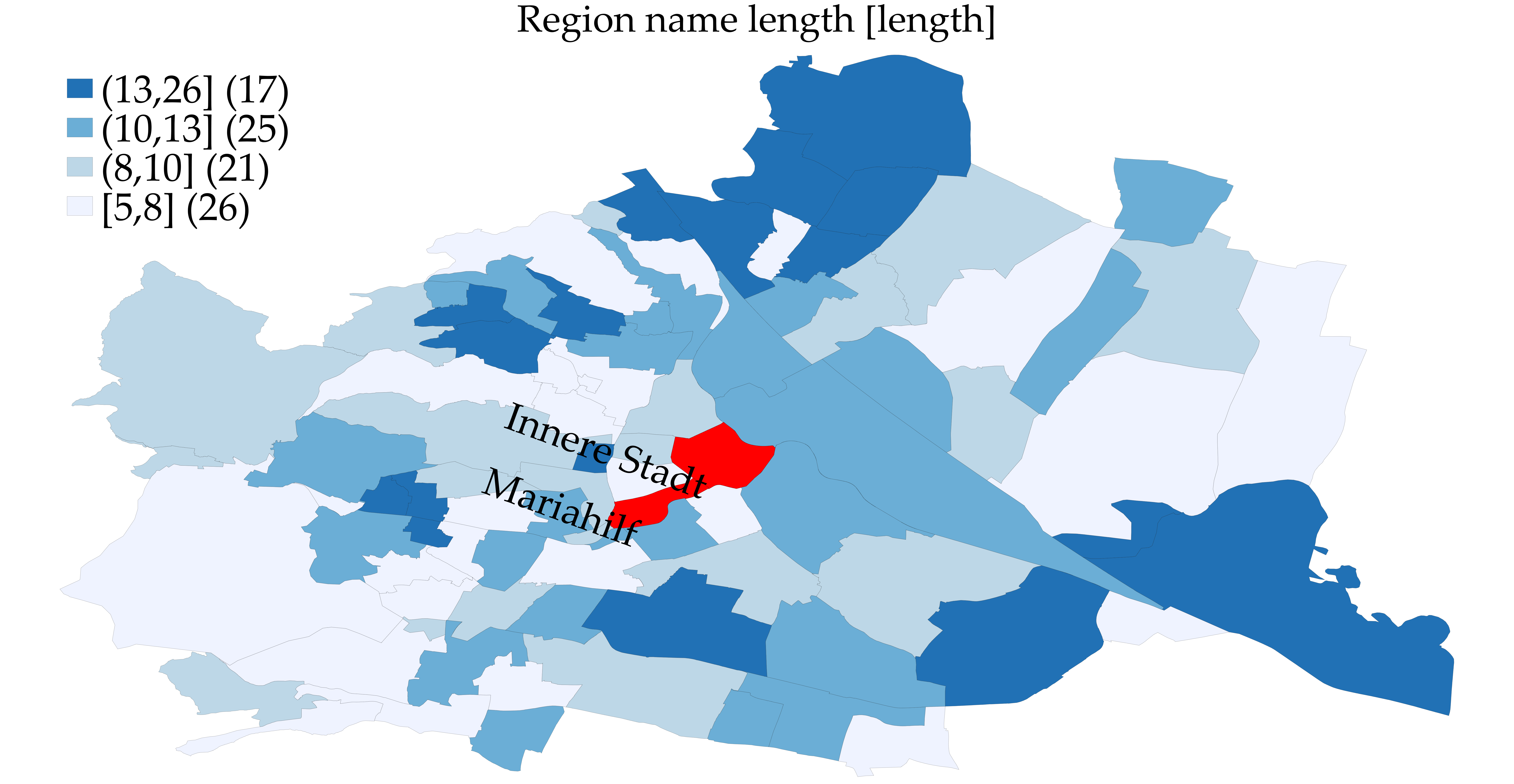

Figure 8: Map of Austria regions’ name length – Zoom on Wien Stadt

The files for replicating these examples are available in the following Dropbox folder. In this short note, I demonstrated simple steps to drawing maps at different level of aggregation with Stata for two different sources (Natural Earth and GADM) of spatial coordinates.

** The author is grateful to Nicholas J. Cox and to an anonymous reviewer for useful remarks that helped me to improve the readability of this note.

The expansion of AI will likely shrink earnings inequality

Visualization of time-varying coefficients

US consumer sentiment and US geopolitical risks

LED Research Seminar

Do Supply Chain Disruptions Matter for Global Economic Conditions?