This post is based on two videos posted by Vasilis Sarafidis on his YouTube channel. In the first one, he presents briefly the theory about the rank condition in CCE estimations. In the second one, he provides some guidance on how to apply the xtdcce2 command, written by Jan Ditzen, to check the rank condition of your static CCE model. The data that I will use has been covered in the following blog:
As explained in the first video, the matrix C, the stacked matrix containing the common factors for all the variables (independent and dependent), has to be full rank to find the matrix F (reminder: a full rank matrix is a matrix where the number of linearly independent rows or columns is equal to the number of rows or columns in the matrix, respectively. In other words, a matrix is said to have full rank if all of its rows or columns are linearly independent).
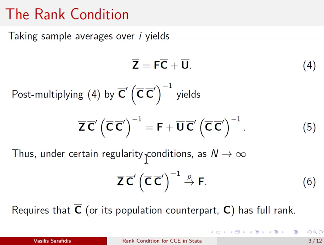
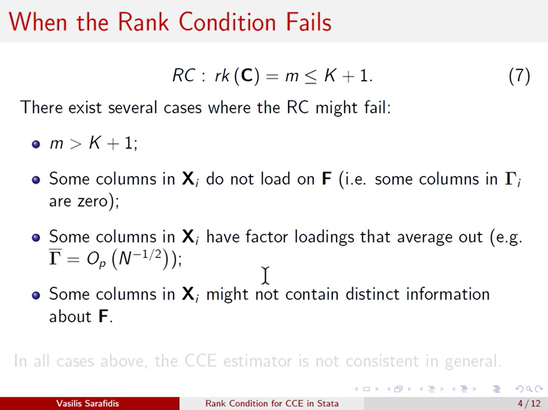
If the matrix C is not of full rank, the CCE estimator is biased. When the number of factors is larger than the number of observables (m > K+1), then the rank condition (RC) fails and C is not invertible. Other cases where the rank condition fails:
Let us apply the estimator of De Vos, Everaert and Sarafidis (2024) to estimate the rank condition with xtdcce2, like explained in the second video:
**# ** Testing the rank condition

*do xr-dynamics_residual_testing.do

xtdcce2  logreer logfeer, crosssectional(_all, rcclassifier)

estat ic, model(logreer logfeer)

xtdcce2  logfeer logreer, crosssectional(_all, rcclassifier)

estat ic, model(logfeer logreer)

label var logreer_cs ///
 "CSA of Log Real Effective Exchange Rates"

label var logfeer_cs ///
 "CSA of Log Fundamental Equilibrium Exchange Rates"

set scheme stcolor

xtline logreer_cs, overlay xtitle("") ///
 name(logreer_cs, replace)

xtline logfeer_cs, overlay xtitle("") ///
 name(logfeer_cs, replace)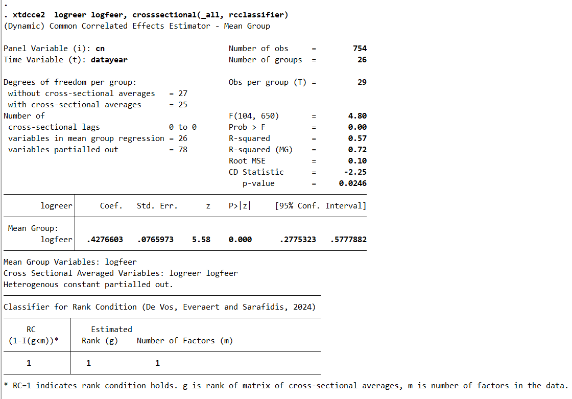
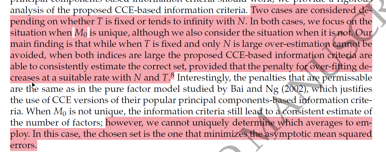
The rank condition is satisfied for my Economic Modelling article of 2015, j.econmod.2015.02.007. I could stop here, but I can use the information criteria to select the right averages in the CCE estimate from Margaritella & Westerlund (2023), ectj/utad009. I thank Peiyun Jiang for signaling me this paper. We are in the case where T and N tends to infinity, since my dataset includes 26 countries observed during 29 years (N = 26; T = 29; N × T = 754). See below:
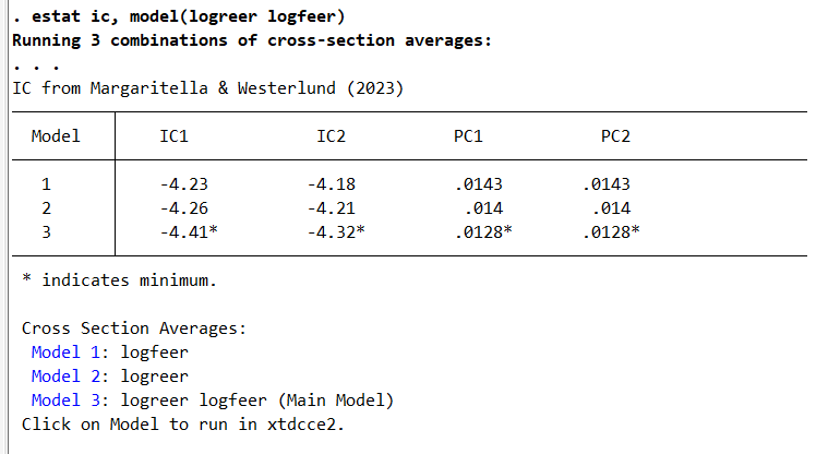
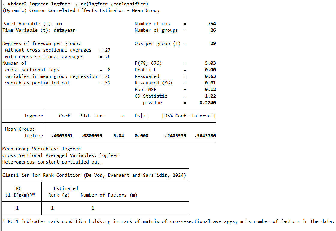
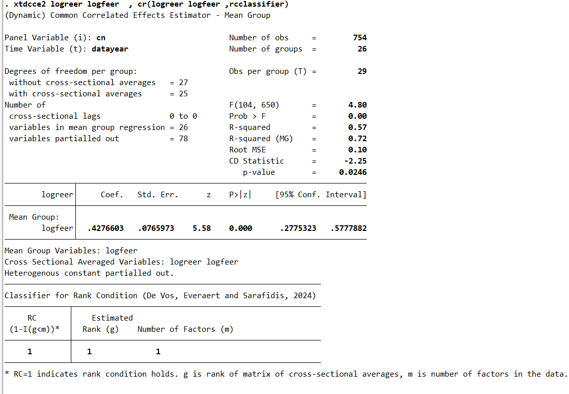
Furthermore, I can compare all these models and the results are very close. Between 0.40 and 0.42. Real effective exchange rates return to their fundamental values, as computed in my FEER approach.
Model 1
Model 2

Model 3
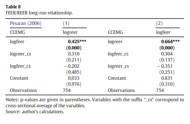
In my article, I used the model 3:
Let us visualize the cross-sectional averages (CSA), while the CSA for the observed exchange rates do not display trends, the CSA for the equilibrium exchange rates has an upward trend, that may be driven by the Balassa-Samuelson effect, as the country sample includes leading emerging markets.
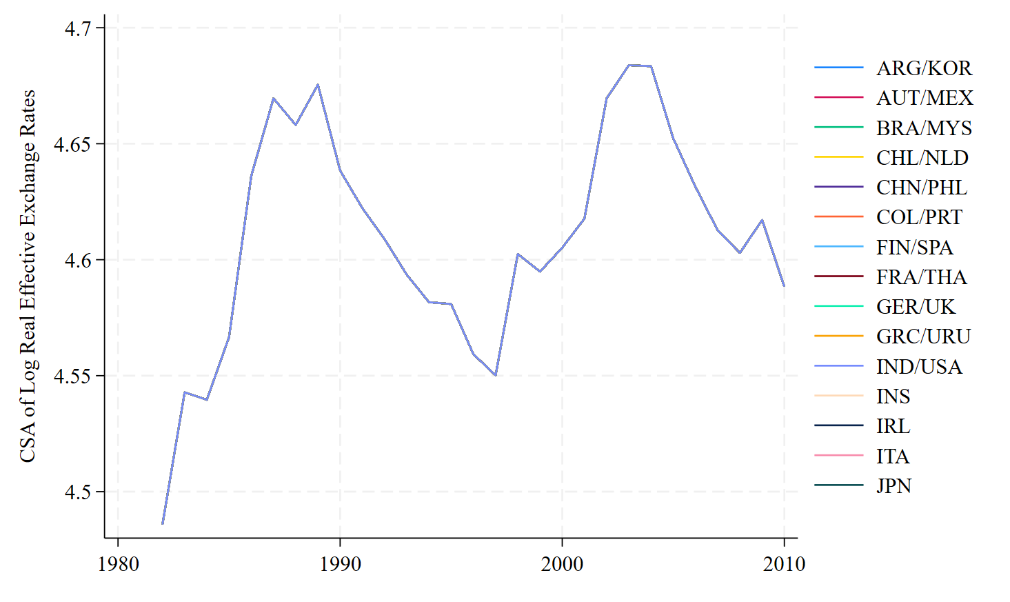
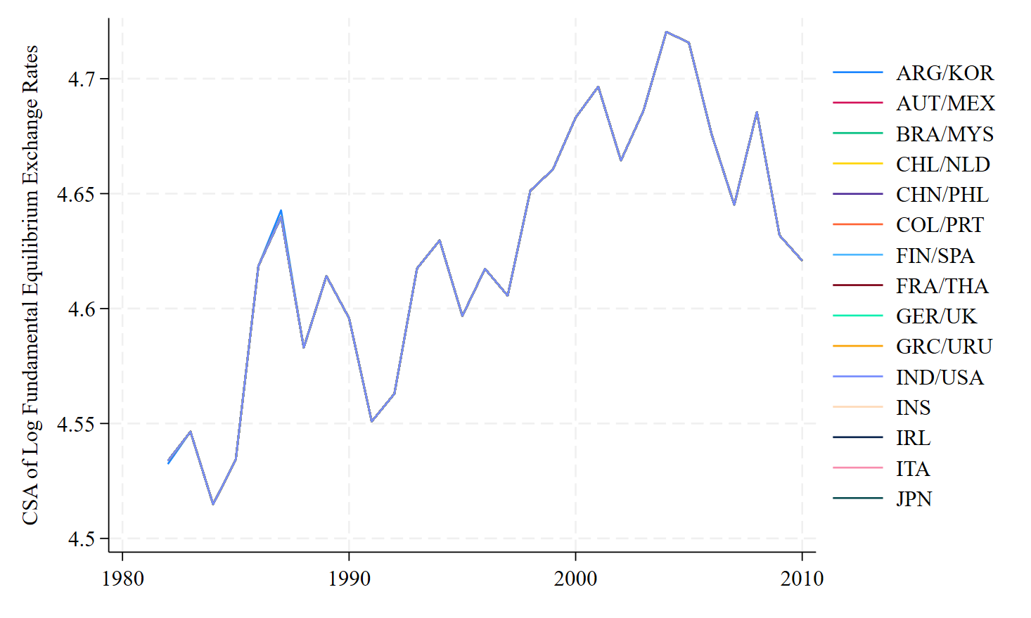
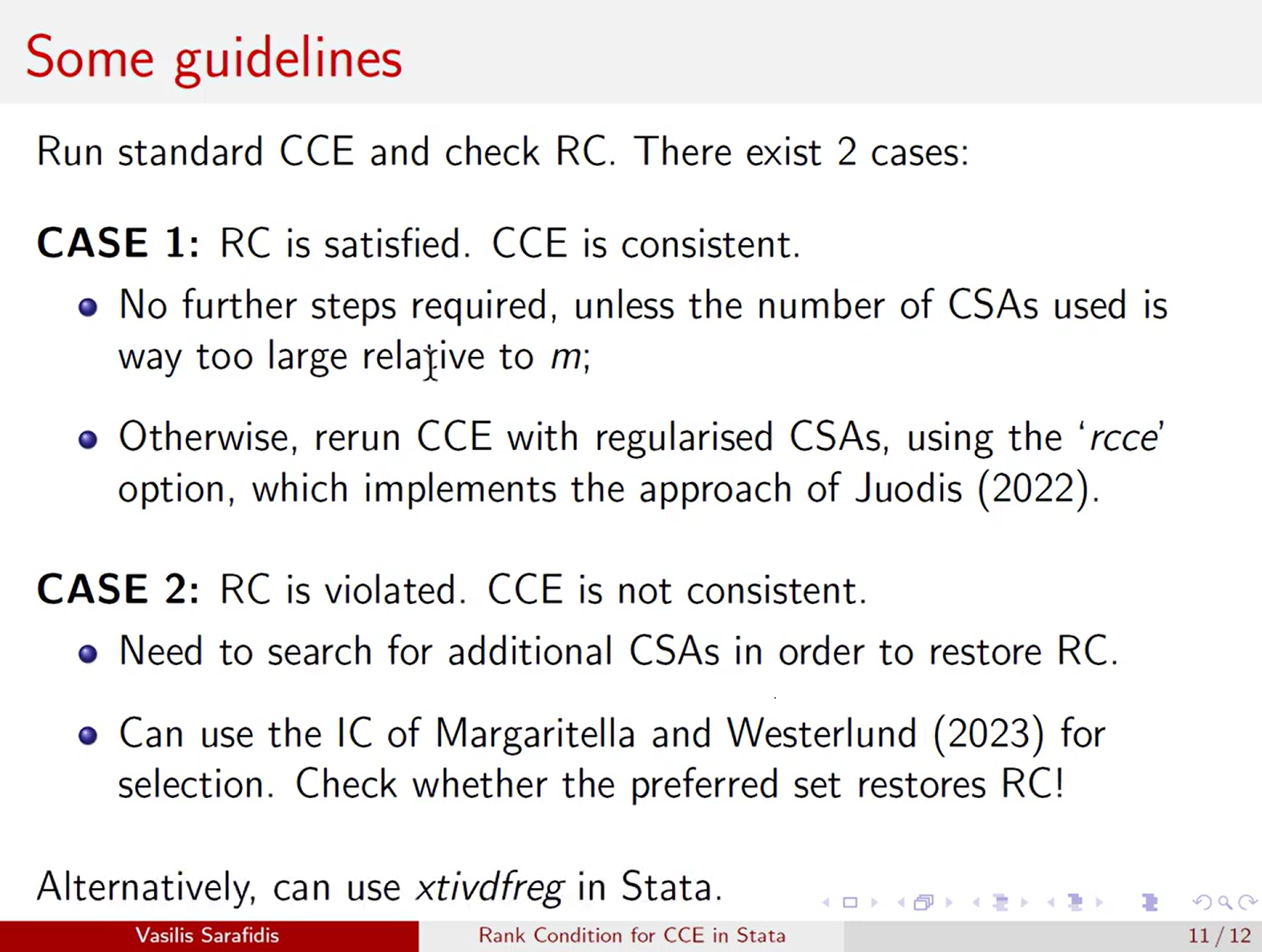
Finally, Vasilis Sarafidis provides some guidelines to check the rank condition (RC) and to select the right CSAs to restore the RC.
If you are keen to learn more about common factors analysis in panel data, I recommend this book:
References
De Vos, I., Everaert, G., & Sarafidis, V. (2024). A method to evaluate the rank condition for CCE estimators. Econometric Reviews, 43(2-4), 123-155.
Ditzen, J. (2018). Estimating dynamic common-correlated effects in Stata. The Stata Journal, 18(3), 585-617.
Ditzen, J. (2021). Estimating long-run effects and the exponent of cross-sectional dependence: An update to xtdcce2. The Stata Journal, 21(3), 687-707.
Margaritella, L., & Westerlund, J. (2023). Using information criteria to select averages in CCE. The Econometrics Journal, 26(3), 405-421.
Saadaoui, J. (2015). Global imbalances: Should we use fundamental equilibrium exchange rates?. Economic Modelling, 47, 383-398.