This post has been inspired by a fascinating discussion with Hiro Ito, Eric Clower and Kamila Kuziemska-Pawlak.
In an old paper of mine (j.econmod.2015.02.007) written in 2015, I tried to answer the following question: Should we use fundamental equilibrium exchange rates to reduce global imbalances? The paper can be considered a reply to an old paper written in 1993 by Su Zhou arguing that exchange rates do not revert to their equilibrium values (10.1007/), as they can be estimated by PPP or FEER models.
After all, if these equilibrium exchange rates any predictive content on real exchange rates, why should we consider them as equilibrium values? They are just desirable counterfactual values for the exchange rates. But, today, I will not enter too deep into these theoretical questions. Instead, I will show the consequences of not introducing common factors into your may have important consequences in your model in terms of prediction.
We will use the data in the article and the codes are available on my GitHub (https://github.com/), I estimate the Pooled Mean Group estimator (s456868) with the following commands:
xtpmg d.logreer d.logfeer, ///
lr(l.logreer logfeer) ec(ec) replace pmg full

Then, I will make the residuals, plot them against the observed values for the variation of the real exchange rate:
capture drop yhat
gen yhat = .
forval cn = 1/26 {
predict temp if cn ==`cn', eq(cn_cn')
replace yhat = temp if cn == `cn'
drop temp
}

gen residuals = d.logreer - yhat

xtline d.logreer yhat
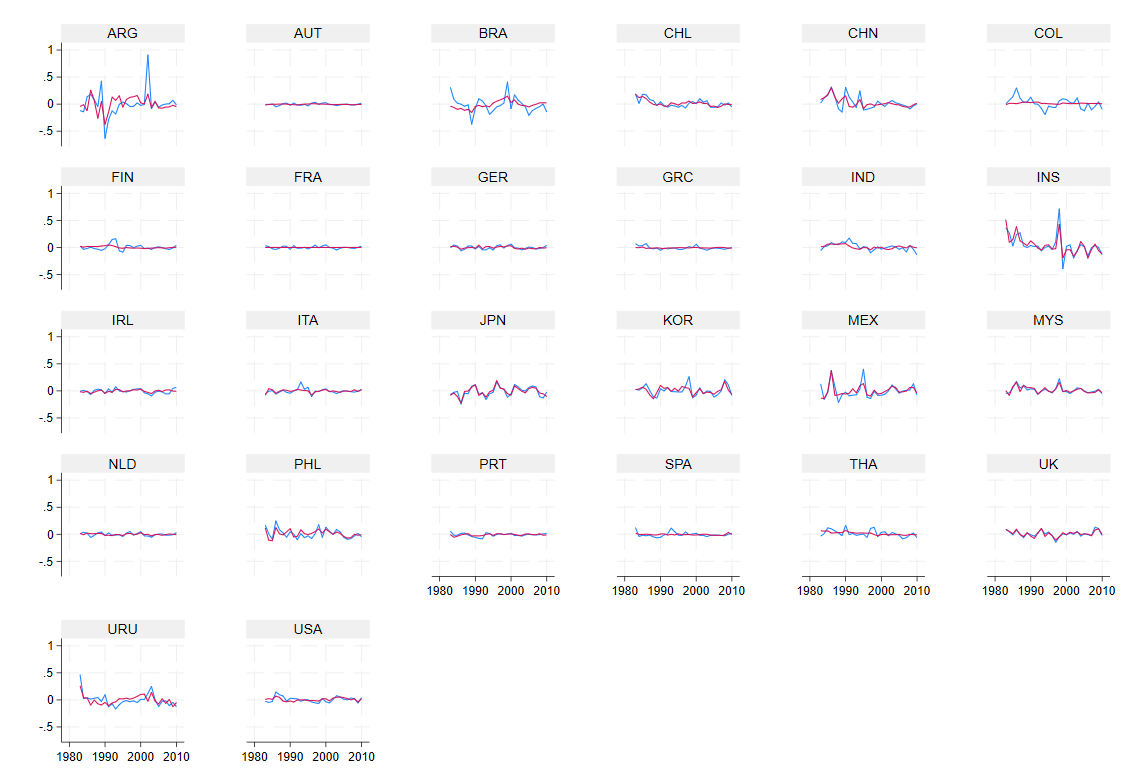
The prediction in red is good, but I may want to test the cross-sectional correlation in the residuals (among other things, we have euro area countries in the sample):
xtcdf residuals
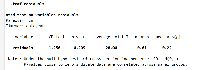
The results are good, but the p-value for the CD test (s458385) is only 20 percent and maybe viewed as low. This panel dataset is balanced and T = 28 (years).
I estimate the same relation between observed exchange rates and equilibrium exchange rates with the cross-sectional averages of the explained and explanatory variables in the short and long run relations:
xtpmg d.logreer d.logfeer d.logreer_cs d.logfeer_cs, ///
lr(l.logreer logfeer l.logreer_cs logfeer_cs) ///
ec(ec) replace pmg full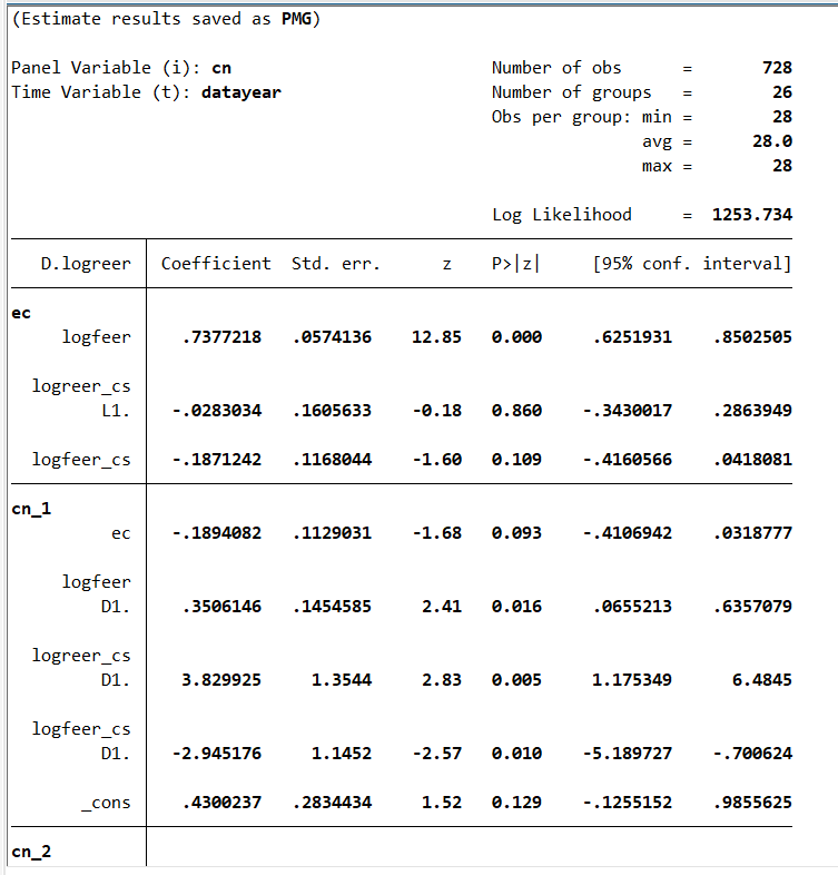
Again, I generate the prediction and plot with the observed value for the variation of the real exchange rate:
capture drop yhat
gen yhat = .
forval cn = 1/26 {
predict temp if cn ==`cn', eq(cn_`cn')
replace yhat = temp if cn == `cn'
drop temp
}

capture drop residuals_cs
gen residuals_cs = d.logreer - yhat

xtline d.logreer yhat

xtcdf residuals_cs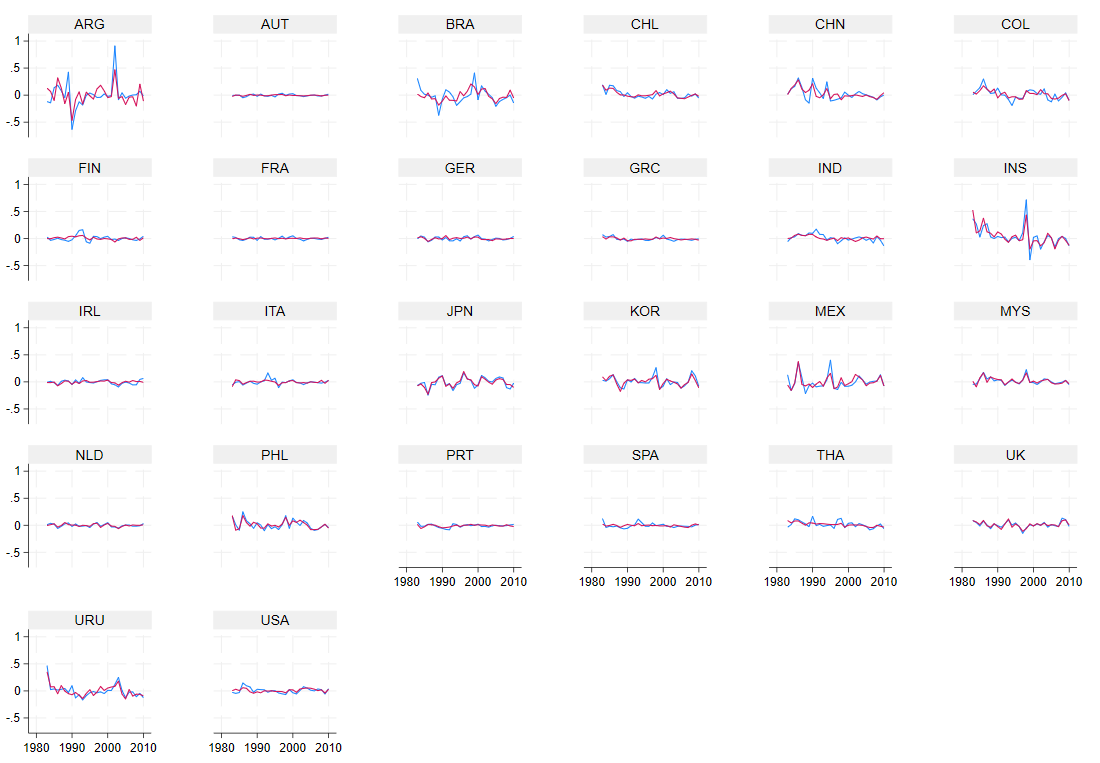
Now, the model seems to have a better fit for some countries, like Argentina and Colombia, for example. It makes sense as the common factor(s) in the exchange has been increasingly influential with financial integration, as explained here (iere.12334). Again, I test the cross-sectional correlation in the residuals:
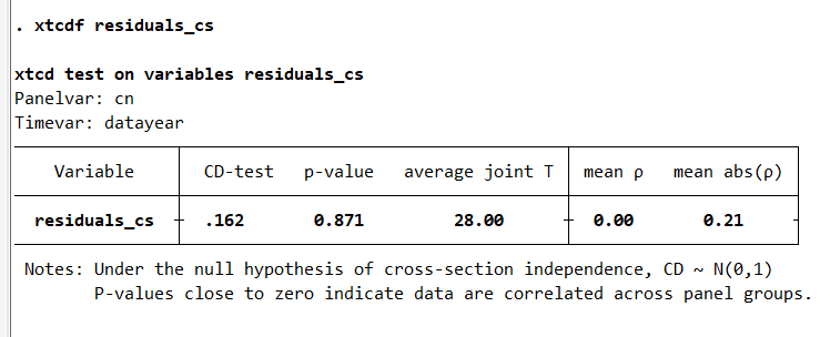
Finally, I can see that the p-value of the CD-test moved from 20 to 80 percent. I can safely conclude that the cross-sectional correlation in the residuals is no longer a big problem in this example.
After excellent remarks made by Rodolphe Desbordes and Jan Ditzen, I was eager to explore the impact of adding a few lags for the cross-sectional averages on the cross-sectional. Rodolphe underlined that it could affect the estimates. I had the chance to meet again Jan at my office yesterday, and we discussed his Stata Journal paper on that question.
Ditzen, J. (2018). Estimating dynamic common-correlated effects in Stata. The Stata Journal, 18(3), 585-617. 1536867X1801800306
We start by estimating the exponent and testing cross-sectional correlation for the variables:
xtcse2 logreer logfeer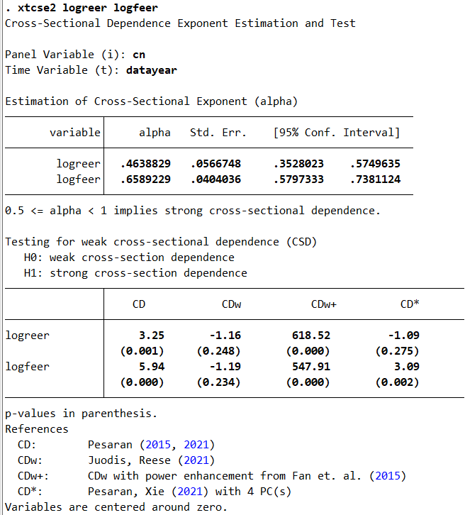
It appears that the variables are impacted by some cross-sectional correlation.
Now, I will estimate the PMG model with the xtdcce2 command. The results will be a bit different as the estimation technique is a bit different (please refer to Ditzen, 2021, for more details and examples).
xtdcce2 d.logreer d.logfeer, lr(L.logreer logfeer) ///
p(L.logreer logfeer) cross(_all) cr_lags(0)  exponent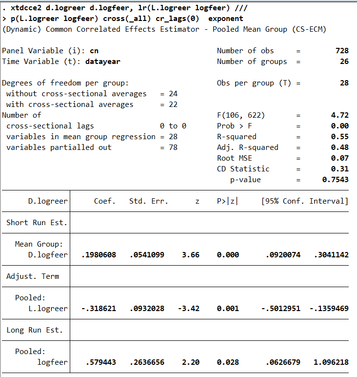
Here, we have 78 variables that are partialed out (26 constants, the cross-sectional averages of logreer_cs logfeer_cs in T, 26×2×1). The number of variables in mean group regression is 28 (26 short-run coefficients, D.logfeer, and 2 cross-sectional averaged variables: logreer logfeer). The CD-test has a p-value of 75%. More on partialing out:
Now, I add two lags for the cross-sectional averages:
xtdcce2 d.logreer d.logfeer, lr(L.logreer logfeer) ///
p(L.logreer logfeer) cross(_all) cr_lags(2) exponent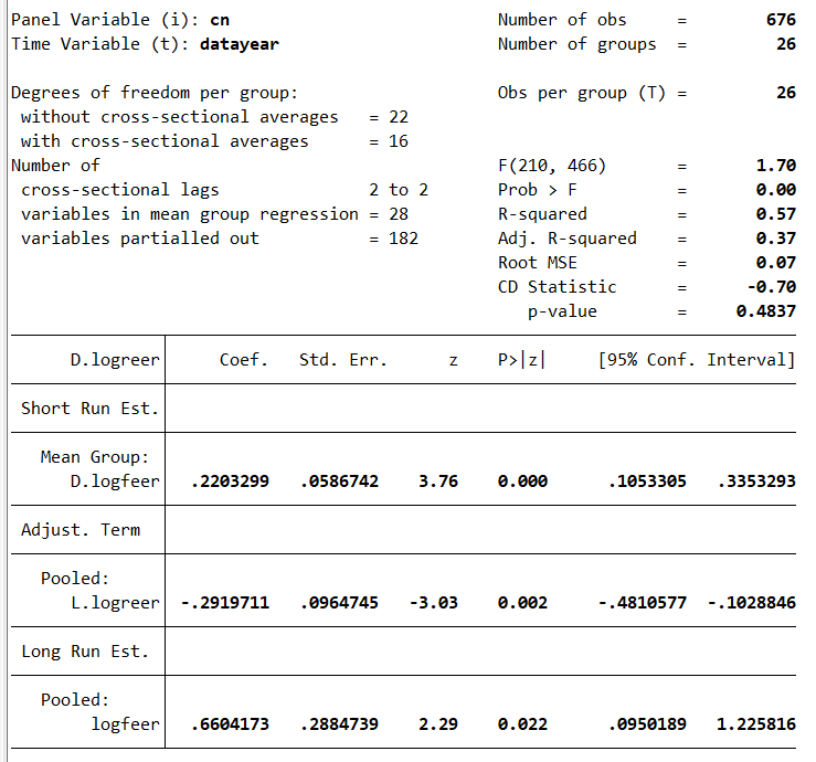
Here, we have 182 variables that are partialled out (26 constants, the cross-sectional averages of logreer_cs logfeer_cs in T, T+1, T+2, 26×2×3). The number of variables in mean group regression is 28 (26 short-run coefficients, D.logfeer, and 2 cross-sectional averaged variables: logreer logfeer). The CD-test has a p-value of 48%.
I now test the strength of the cross-sectional dependence after this estimation:
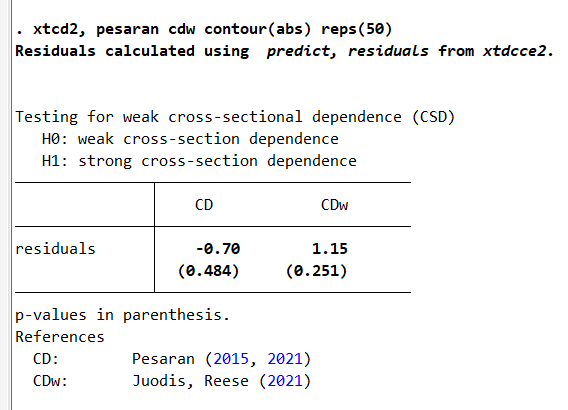
The conclusions are qualitatively similar to those with fewer cross-sectional averages. More about common factors:
As we have seen in this blog, it is possible to test cross-sectional correlation of the residuals after using the xtpmg command in Stata. More importantly, we can intuitively understand the consequences of cross-sectional correlation in the residuals. The files for replicating the results in this blog are available on my GitHub.