During my seminars of Applied Econometric with Stata in the Faculty of Economics and Management at the University of Strasbourg, I always tell to my students that the concept of size and power are very important in statistics and in econometrics. Indeed, size (Type I error) and power (1-Type II error) analyses are often used to evaluate the statistical properties for a new test or for a newly proposed estimator. The size and power will be affected by the sample size, but also by the effect size. The objective for the econometricians is to achieve a high power and a small size with a few observations. But, can we observe a trade-off between size and power in small samples?
I asked the AI research assistant, if it can define a power analysis:
In the context of hypothesis testing, power and size are important concepts related to the performance of the test. Specifically, for a two-sample t-test, which compares the means of two groups to determine whether there is a significant difference between them, these concepts can be defined as follows:

Power: Power is the probability that a test will correctly reject the null hypothesis when the alternative hypothesis is true. In other words, it measures the ability of the test to detect an actual effect (i.e., a true difference between the two groups). A higher power means that the test is more likely to identify a significant difference when one exists. The power of a test is influenced by factors such as sample size, effect size (the magnitude of the difference between the groups), and the significance level.

Size (or Significance Level): The size of a test, commonly denoted by alpha (α), is the probability of rejecting the null hypothesis when it is true. This is also known as a Type I error, or a false positive. The significance level is a threshold that determines how strong the evidence against the null hypothesis must be before it can be rejected. Commonly used significance levels are 0.05 and 0.01, which correspond to a 5% and 1% chance of making a Type I error, respectively.

For a two-sample t-test, the goal is to strike a balance between the power and size of the test. Ideally, you want to have high power to detect true effects and a low significance level to minimize the chances of making Type I errors. Increasing the sample size is one way to achieve higher power without increasing the risk of Type I errors.
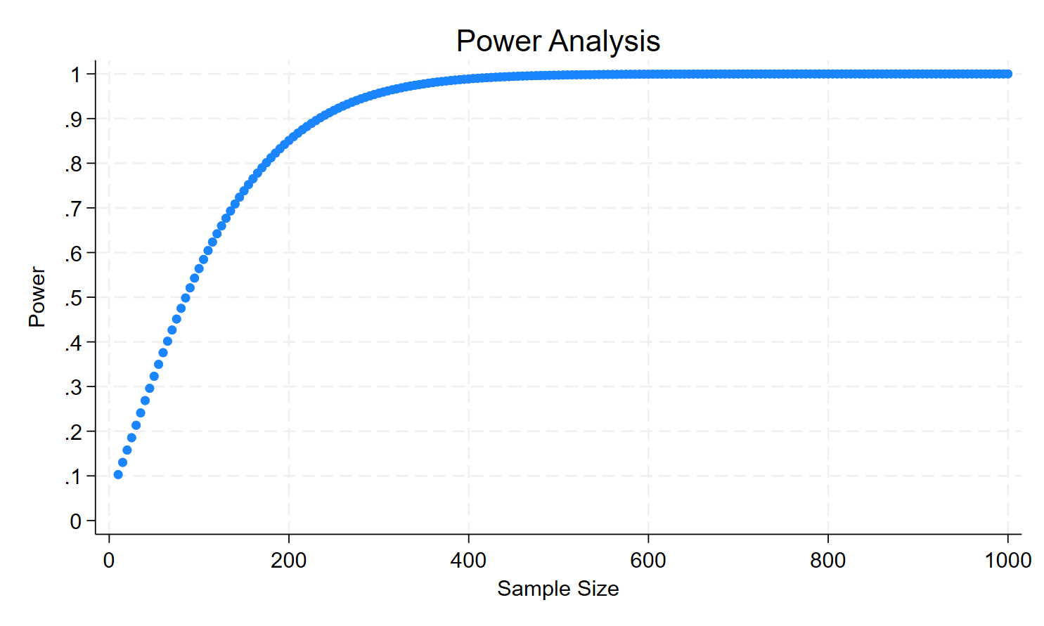
I will come back on the code that produces this last figure, but we clearly see that from 200 observations, the test achieves a reasonable power of 80 percent.
Now, we can look at the Stata code produced by the AI (I made a few iterations with ChatGPT 3.5 and 4):
cls
clear

* Set up parameters for power analysis
local alpha = 0.05   // significance level
local effect_size = 0.3 // expected effect size

* Set up range of sample sizes
local min_n = 10
local max_n = 1000
local step_n = 5

* Calculate the number of steps
local num_steps = round((`max_n' - `min_n') / `step_n' + 1)

* Create dataset with sample sizes
clear
set obs `num_steps'
gen sample_size = .
gen power = .
local i = 1

* Define a program to calculate power for a given sample size
capture program drop calc_power
program calc_power, rclass
    args n alpha effect_size
    sampsi 0.0 `effect_size', sd(1.0) n(`n') alpha(`alpha')
    return scalar power = r(power)
end

* Calculate power for each sample size, store and display the results
forvalues n = `min_n'(`step_n')`max_n' {
    calc_power `n' `alpha' `effect_size'
    local power = r(power)
    display "Sample size: " `n' " Power: " `power'
    replace sample_size = `n' in `i'
    replace power = `power' in `i'
    local i = `i' + 1
}
Since we have a t-test for two sample means, we want to detect that the means are different. We build on the Stata command sampsi and we write a program that will help us compute the power. Afterward, we post the power and the sample size into variables to draw the figure.
Before looking at the ‘program’ part code, a small piece of advice: do not run the code line by line when you use the local command (it will produce an r(198) syntax error). Now, it could be quite pedagogical to explain the ‘program’ part of the code:
/*
capture program drop calc_power: This line ensures that if a program named calc_power already exists, it will be removed before the new program is defined. capture prevents Stata from displaying an error message if the program does not exist.
program calc_power, rclass: This line starts the definition of a new program named calc_power. The rclass option specifies that the program will return results in the r() return list, which can be accessed after the program is executed.
args n alpha effect_size: This line specifies that the program takes three arguments: n (sample size), alpha (significance level), and effect_size (expected effect size). These arguments will be passed to the program when it's called.
sampsi 0.0 effect_size', sd(1.0) n(n') alpha(alpha'): This line calls Stata's built-in sampsi` command to perform a sample size and power analysis. The command calculates the power for a two-sample t-test with the given effect size, sample size, and significance level, assuming a standard deviation of 1.0 for both groups.
return scalar power = r(power): This line stores the calculated power from the sampsi command in a scalar named power. The r(power) refers to the power value that is stored in the r() return list after running the sampsi command. By assigning the value to a scalar in the return list, it can be easily accessed outside the program.
end: This line marks the end of the calc_power program definition.
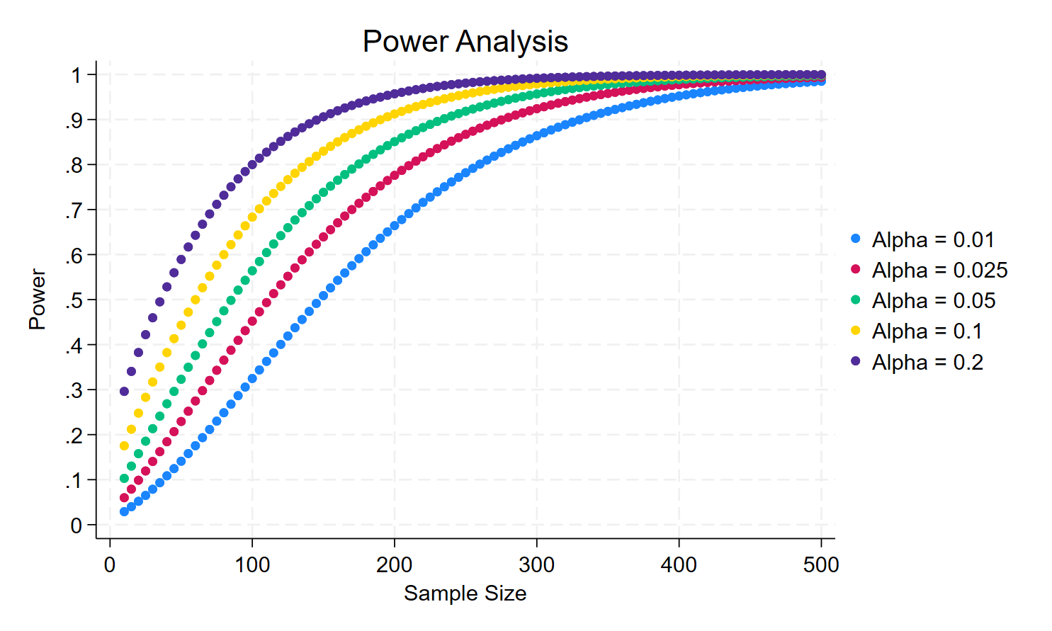
*/Now, I can try to use the previous code to draw the power for different sizes (Type I error). Unsurprisingly, we will observe that there is a trade-off between size and power (1-Type II error). For less than 300 observations, we need to accept a loss of power if we want a smaller size in order to detect a difference between the mean in each of the sample of 0.3. If we have 100 observations, we want a size = 0.01, we need to accept that the power will be only of 30%.
Suppose that the effect size (here, the difference between the sample means) is now smaller, say 0.15, what would be the result?
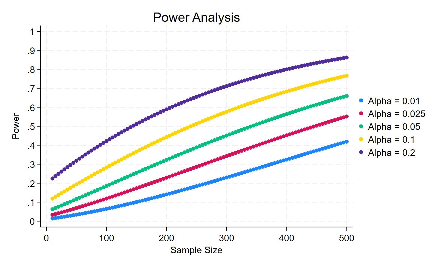
The trade-off is even worse, you have to accept a very low power (below 10%) if you want to have the same size.
Now, we increase the effect size to 0.45. What would be the result?
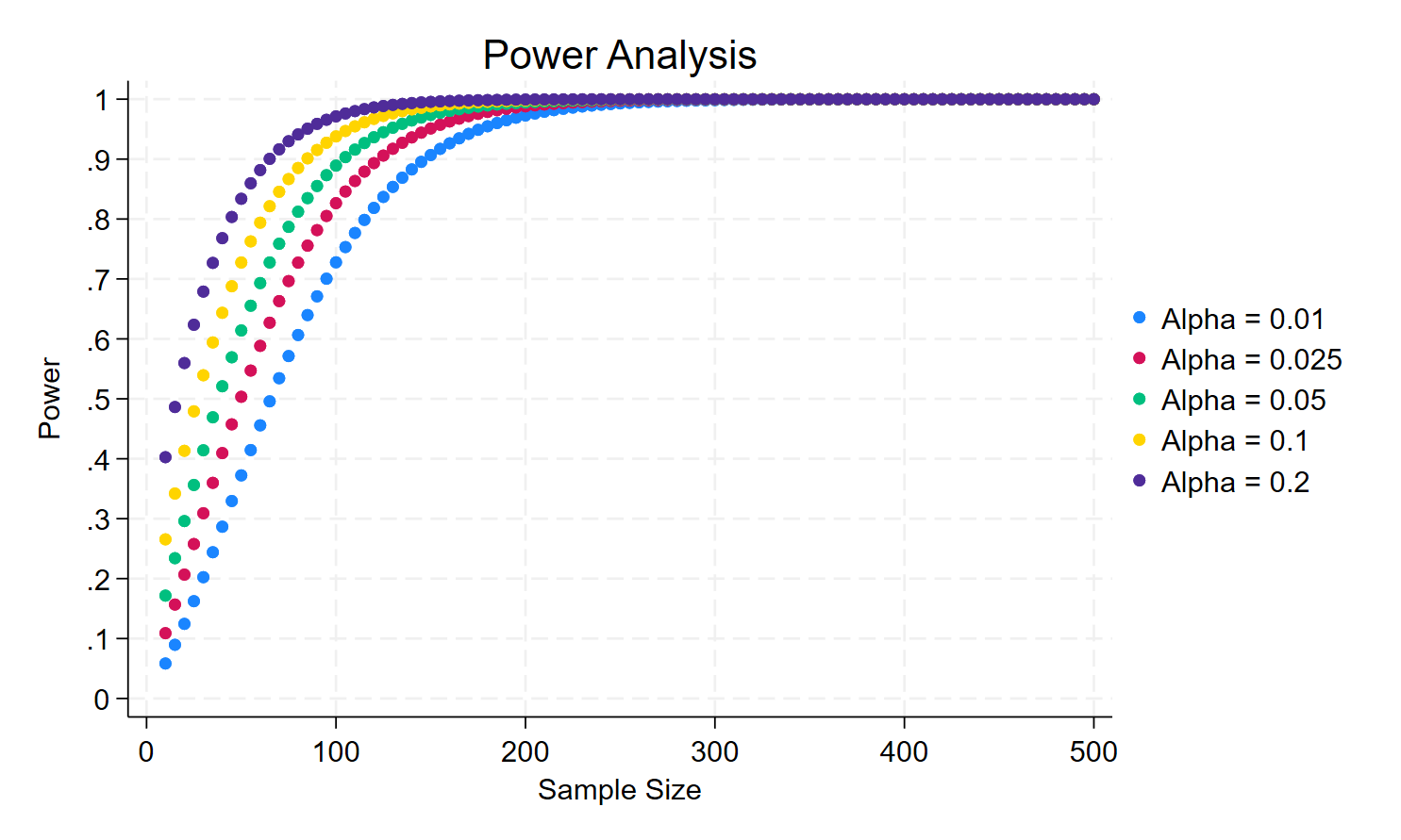
Now, the trade-off between size and power has disappeared.
Conclusion: if you are using a small sample and you intend to detect small effects, you have to be careful about the trade-off between size and power.
cls
clear

* Set up parameters for power analysis
local alphas = "0.01 0.025 0.05 0.1 0.2" // different significance levels
local effect_size = 0.45 // expected effect size

* Set up range of sample sizes
local min_n = 10
local max_n = 500
local step_n = 5

* Calculate the number of steps
local num_steps = round((`max_n' - `min_n') / `step_n' + 1)

* Define a program to calculate power for a given sample size and alpha
capture program drop calc_power
program calc_power, rclass
    args n alpha effect_size
    sampsi 0.0 `effect_size', sd(1.0) n(`n') alpha(`alpha')
    return scalar power = r(power)
end

* Create a dataset with sample sizes
clear
set obs `num_steps'
gen sample_size = .

* Generate variables for power at different alpha levels
foreach a in `alphas' {
    local a_underscored: subinstr local a "." "_", all
    gen power_alpha_`a_underscored' = .
}


* Loop through each alpha value and calculate power for each sample size
foreach a in `alphas' {
    local a_underscored: subinstr local a "." "_", all
    local i = 1
    forvalues n = `min_n'(`step_n')`max_n' {
        calc_power `n' `a' `effect_size'
        local power = r(power)
        display "Alpha: " `a' " Sample size: " `n' " Power: " `power'
        replace sample_size = `n' in `i'
        replace power_alpha_`a_underscored' = `power' in `i'
        local i = `i' + 1
    }
}


* Generate a scatter plot of power vs sample size for all alphas
twoway (scatter power_alpha_0_01 sample_size, msymbol(O) msize(small) mcolor(black)) ///
       (scatter power_alpha_0_025 sample_size, msymbol(O) msize(small) mcolor(blue)) ///
       (scatter power_alpha_0_05 sample_size, msymbol(O) msize(small) mcolor(red)) ///
       (scatter power_alpha_0_1 sample_size, msymbol(O) msize(small) mcolor(green)) ///
       (scatter power_alpha_0_2 sample_size, msymbol(O) msize(small) mcolor(orange)), ///
        xscale(range(`min_n' `max_n')) ylabel(0(0.1)1) ///
        xtitle("Sample Size") ytitle("Power") ///
        title("Power Analysis") ///
        legend(order(1 "Alpha = 0.01" 2 "Alpha = 0.025" 3 "Alpha = 0.05" ///
                    4 "Alpha = 0.1" 5 "Alpha = 0.2")) ///
        graphregion(color(white)) plotregion(color(white))


* Save the graph as a PNG file
graph export "power_analysis_plot_combined.png", replace

save power, replace
Please note that the files for replicating this blog are (or will be) available here: https://github.com/