Panel Data Econometrics: Common Factor Analysis for Empirical Researchers [Update]

Edit: It is an honor to be included on the companion website of Professor Sul: https://personal.utdallas.edu/~dxs093000/book/panel.htm

During this summer, I decided to explore and to understand the concept of common factors in panel data econometrics, which are a very important thing, in the exchange rate literature for example. These co-mouvements sometimes have a high explanatory power, even more than those of the fundamental variables.

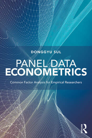
I read this wonderful book, Panel Data Econometric: Common Factor Analysis for Empirical Researchers, written by the Professor Donggyu Sul. This book has many merits. First, the paper has been written for empirical researchers with a companion website with STATA, MATLAB and GAUSS routines for chapter 3 to 7. I really believe that practicing econometrics is the best way to learn and digest econometric theory. Besides, I am more of a STATA user, and it was very nice to learn how to transpose my STATA knowledge to GAUSS and MATLAB, which are very useful to implement econometrics due to their management of the matrix language.

When I was at the beginning of my PhD and reading some IMF working papers, I was always wondering the sense of including both individual fixed effects and time individual fixed effects in a panel of macroeconomic variables or macro-financial variables. In these IMF working papers, they used individual fixed effects or time fixed effects, but never both in the same regression. Indeed, it makes sense to include individual fixed effects if you want to examine the within countries correlations. Besides, it makes senses to include time fixed effect if you intend to investigate the between countries correlation.

In the first chapter of the book, the basic structure of panel data is clearly explained and the Professor Sul provides the answer. When you include both individual and time effects, it remains the third term of the decomposition equation below, a purely idiosyncratic term. The panel data can be decomposed in (i) a time-invariant individual specific variables, (ii) a time-varying common variables, (iii) a time-varying individual specific variables. The second term is the common factor and the third term is the idiosyncratic term.

y_{it}=a_i+\theta_t+y^o_{it}

So, what does it mean to include both individual and time fixed effects in panel data regressions? If you are interested in explaining the national or the aggregate behavior, you should not eliminate the common factors (or introduce time fixed effects)! The chapter also provides three ways to interpret the common factors: (i) aggregation, (ii) common shocks, and (iii) central tendency.

The chapter 2 provides an overview about the different statistical models for cross-sectional dependence. For example, spatial dependence can be considered as weak dependence because the cross-sectional correlation fades away when the physical distance increases. Besides, the cross-sectional dependence changes depending on the ordering of the statistical units in the panel!

The chapter 3 explains and describes the algorithms used to identify the number of the common factors. For example, you should use first differenced and standardized variables to identify the correct number of common factors.

The chapter 4 provides methods to estimates the common factors, the principal component analysis and the cross-sectional average. The cross-sectional average estimator is more efficient when the variance of the idiosyncratic component is not so large. The cross-sectional average estimator remains the same in level and in first difference. The idiosyncratic components can be extracted after the estimation of the common factor. It also presents a nice reminder about the measurement of accuracy. In general, the uncertainty between the estimate (sample) and the parameter (population) is usually reduced when the number of observations increases.

The chapter 5 presents some very interesting ways to identify the common factors. Indeed, the latent (true) factors can be different from the estimated factor. The asymptotically weak factors approach is very interesting since it tests directly the presence of common factor in the idiosyncratic term. Basically, if you have the correct number of factors and that you have the true factors, then the idiosyncratic term should be free of cross-sectional dependencies.

The chapter 6 provides very good insights on how to interpret dynamic and static relationships. It provides the bias (difference between the estimate (sample) and the true value of the parameter (population)) for five estimators (cross-sectional regressions, pooled OLS, time series regression and fixed effects regressions, and between-group estimations) when the dynamic and static relationships differ, under cross-sectional independence and dependence.

The chapter 7 magisterially distinguishes three notions of economic convergence, namely: beta-convergence, relative, sigma convergence. A formal test of sigma-convergence is presented and discussed (see Kong, Phillips and Sul, 2018 for more detail, codes available on the Professor Sul’s website).

In the appendix, Chapter 8 presents some useful reminders on basic panel regressions and the use (and misuse) of the two-way fixed effect estimator.

In a nutshell, I would like to highly recommend this book not only for PhD student, but also for empirical researchers that want to keep up with the recent developments of panel data econometrics. I can’t wait for the next editions!