Today, I propose an update of the following blog. So I recommend reading it before dive in this blog. Adding shaded areas is very simple with EViews, but not so simple in Stata. I will show that you can use twoway and raera to simplify the addition of shaded areas in a Stata graph.
Key takeaways
- Simplify recession shading in Stata with
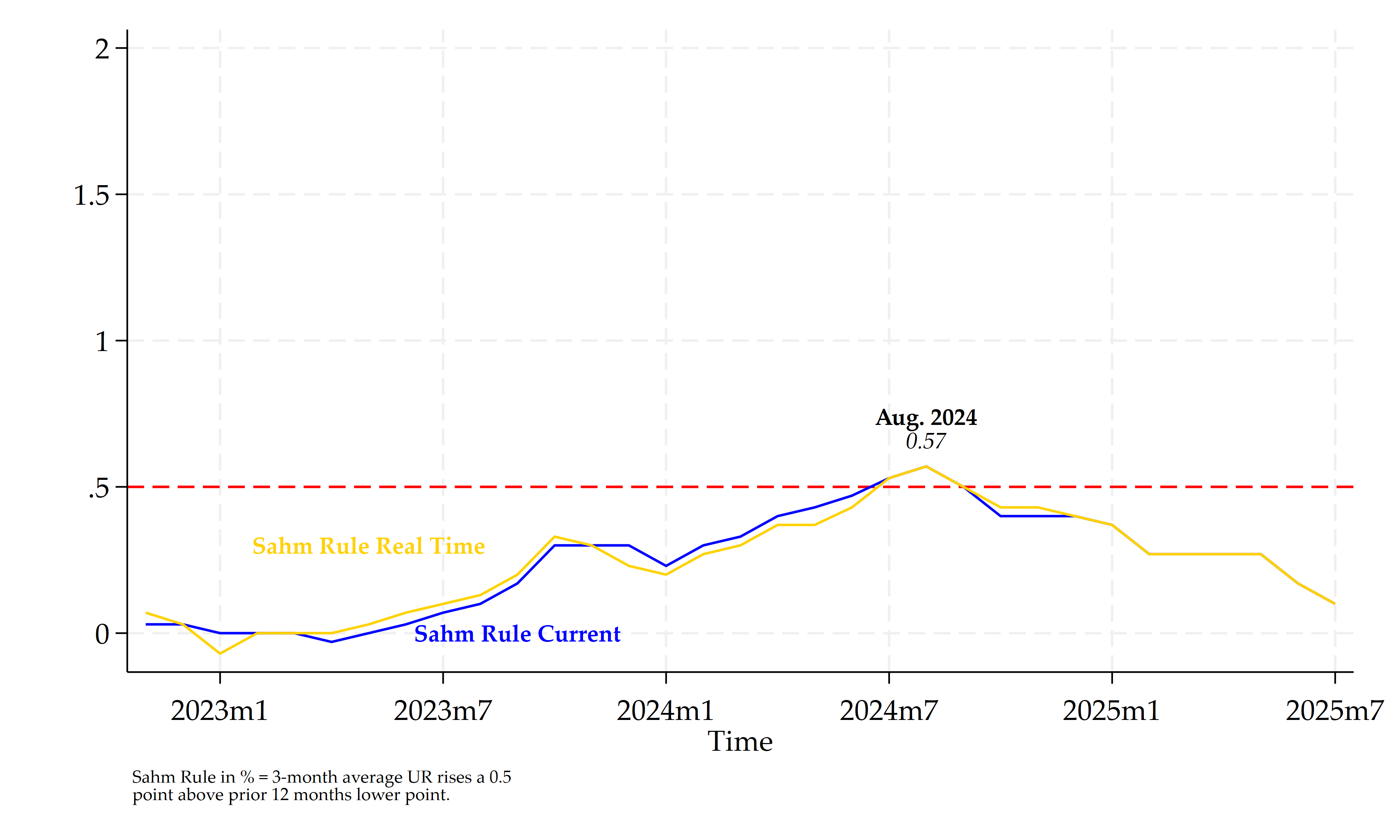
rarea; efficient coding improves clarity in time series analysis. - The Sahm Rule broke in Aug. 2024, reminding us that economic “laws” are time-varying and lack physics-like universality.
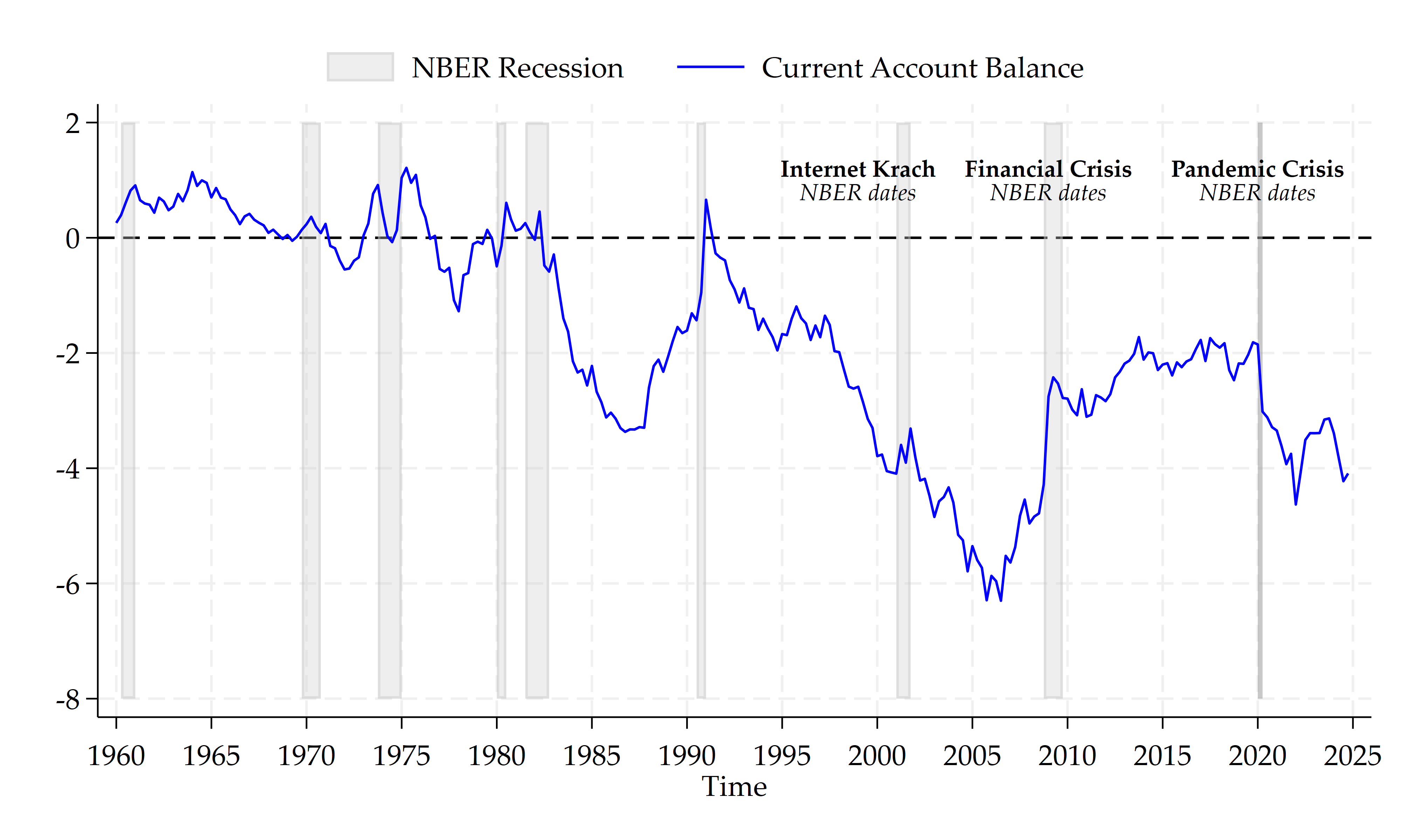
- US current account balance shows no systematic pattern before recessions, unlike the GFC or earlier downturns.
- Using locals
ytandybstreamlines shaded bands, ensuring consistent graph scaling and visual accuracy. - Updated graphs combine coding refinements with economic insights, bridging method and interpretation.
I update the graphs for the Sahm Rule and for the current account balance. In August 2024, the Sahm Rule has been been broken.
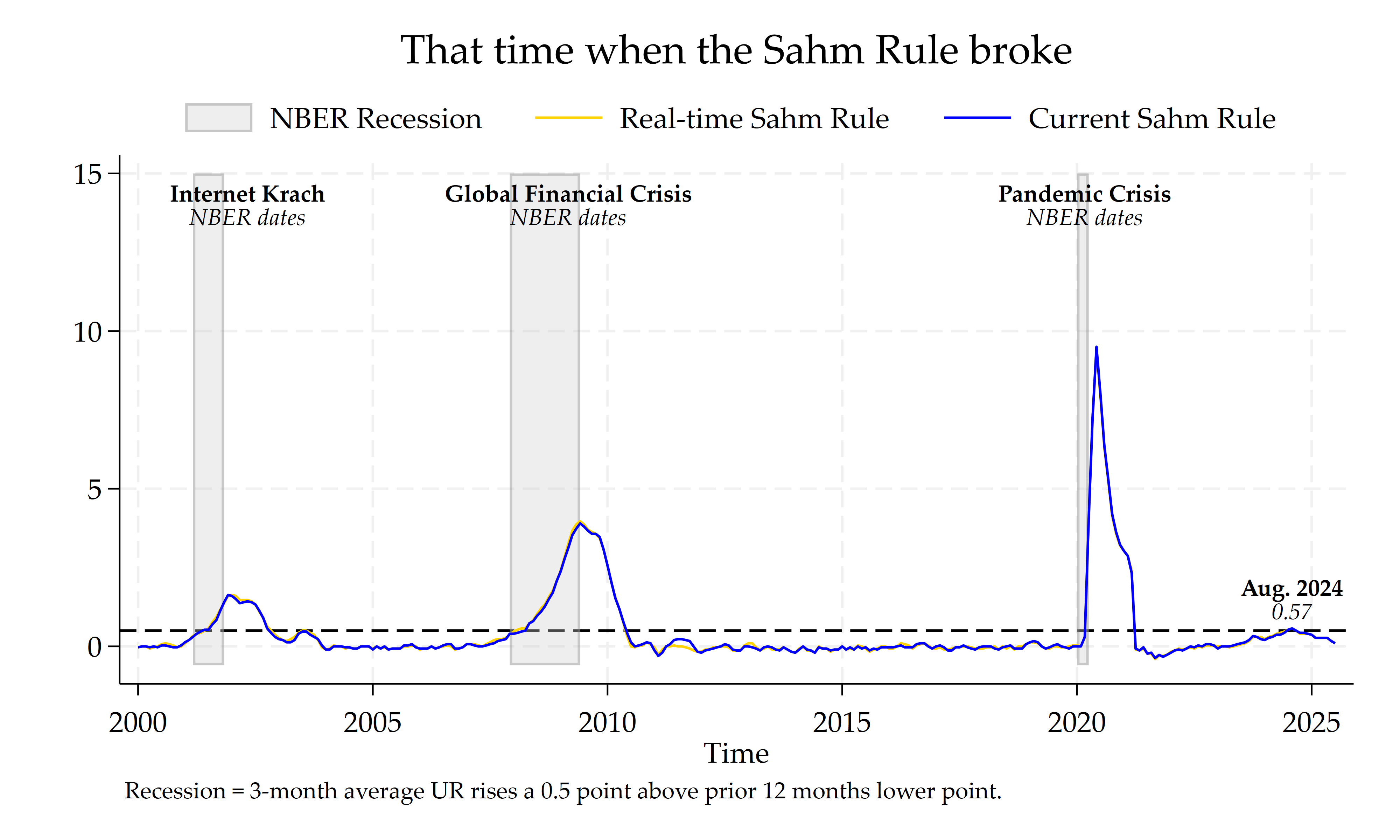
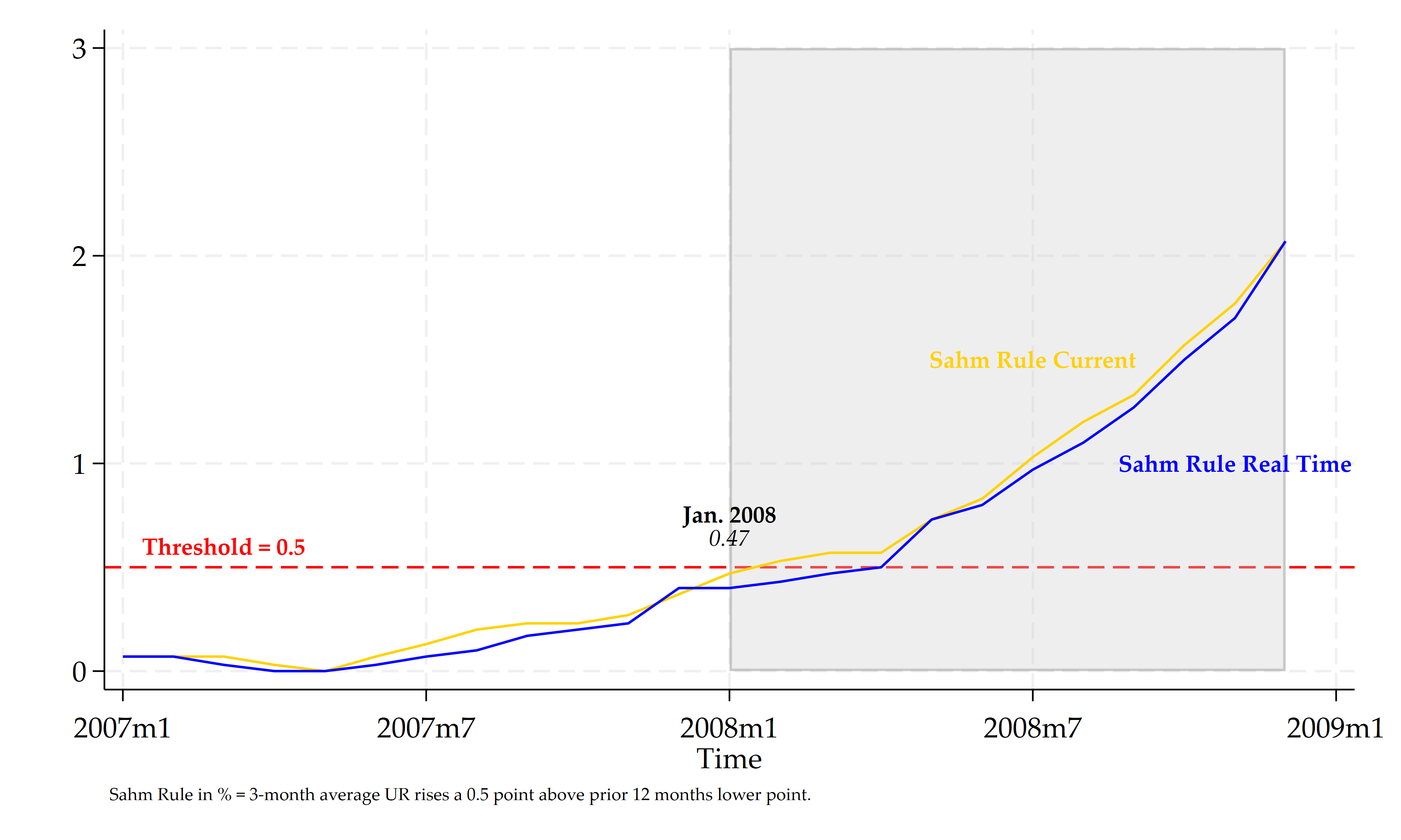
Usually, crossing the threshold of 5 percent was followed by an NBER recession, like before the GFC.
It was not the case in August 2024, this is not surprising. In Economics, what we call “law” have not the same epistemological status as the Physicists discover about the cosmos. In Economics as in other social sciences, causality is difficult to establish and is, often, time-varying..
What we can see here is that we do not have a systematic behavior of the US current account balance before recessions, see some reflections about it here.
The main improvement is in this part, the locals yb and yt will be used in the rarea part of the code:
// Prep shaded bands & y-limits
summarize USAB6BLTT02STSAQ
scalar ytop = 2
scalar ybot = -7

cap drop y0
cap drop yM

cap gen double y0 = ybot
cap gen double yM = ytop

// y-positions for arrows & labels
local yb   = `=ybot'
local yt   = `=ytop'
The full code is reproduced below:
**# ****** Shaded areas more efficiently *************************

// Choose your working directory

cd "C:\Users\jamel\Dropbox\stata\shading"

// An interesting blog on the topic

/*
https://blog.stata.com/2020/02/13/adding-recession-
shading-to-time-series-graphs/
*/

// Choose your scheme

set scheme stcolor

// Add your API key

/*
set fredkey 01b83643a9864a8f910a499e5022b2d6, permanently
*/

// Search the series and downlaod the data with an API key

/*
fredsearch sahm rule
*/

import fred SAHMREALTIME SAHMCURRENT, clear
display=td(01jan2000)
keep if daten>=td(01jan2000)
generate datem = mofd(daten)
tsset datem, monthly

label variable SAHMREALTIME ///
 "Real-time Sahm Rule"

label variable SAHMCURRENT ///
 "Current Sahm Rule"

label variable datem ///
 "Time"

// Description:
/*
https://research.stlouisfed.org/publications/research-news/
fred-adds-sahm-rule-recession-indicators
*/

/*
Econbrowser blog: https://econbrowser.com/archives/2024/01/are-we-in-recession-the-sahm-rule-now-2007
*/

// Display dates
display tm(2001m3)
display tm(2001m11)
display tm(2007m12)
display tm(2020m1)
display tm(2020m4)

// Prep shaded bands & y-limits
summarize SAHMCURRENT
scalar ytop = ceil(r(max)/1)*1.5
scalar ybot = (r(min)/1)*1.5

cap drop y0
cap drop yM

cap gen double y0 = ybot
cap gen double yM = ytop

// y-positions for arrows & labels
local yb   = `=ybot'
local yt   = `=ytop'

// Recession dates (Improved)
cap gen byte band_greatinfl = ///
 inrange(datem, tm(2001m3), tm(2001m11))
cap gen byte band_gfc = ///
 inrange(datem, tm(2007m12), tm(2009m6))
cap gen byte band_2020s = ///
 inrange(datem, tm(2020m1), tm(2020m4))

// Declare your time series and first graph

tsset datem

tsline SAHMCURRENT SAHMREALTIME, tlabel(, format(%tmCCYY))
graph rename sahm, replace

*set scheme white_jet

twoway ///
     rarea y0 yM datem if band_greatinfl, ///
        color(gs12%35) lcolor(gray) || ///
     rarea y0 yM datem if band_gfc, ///
        color(gs12%35) lcolor(gray) || ///
     rarea y0 yM datem if band_2020s, ///
        color(gs12%35) lcolor(gray), || ///
  (tsline SAHMCURRENT SAHMREALTIME, lcolor(gold blue) ///
   title("That time when the Sahm Rule broke") ///
   xlabel() ///
   tlabel(, ///
   format(%tmCCYY))), yline(0.5) ///
   legend(order(2 "NBER Recession" ///
           4 "Real-time Sahm Rule" 5 "Current Sahm Rule") ///
           pos(12) ring(1) col(3) ///
           region(lstyle(none))) ///
  text(14 508 "{bf:Internet Krach}" "{it:NBER dates}", ///
  size(small)) ///
  text(14 590 "{bf:Global Financial Crisis}" ///
  "{it:NBER dates}", size(small)) ///
  text(14 722 "{bf:Pandemic Crisis}" "{it:NBER dates}", ///
  size(small)) ///
  text(1.5 775 "{bf:Aug. 2024}""{it:0.57}", size(small)) ///
  note("Recession = 3-month average UR rises a 0.5 point above prior 12 months lower point.", size(small)) ///
 graphregion(margin(l+2 r+2))

// Export the graph in two different formats

graph rename sahmrule, replace
graph export sahmrule.png, as(png) ///
 width(4000) replace
graph export sahmrule.pdf, as(pdf) ///
 replace

// Run everthing between preserve and restore
***
preserve

keep if datem>=tm(2007m1) & datem<=tm(2008m12)

// Prep shaded bands & y-limits
summarize SAHMCURRENT
scalar ytop = ceil(r(max)/1)*1
scalar ybot = (r(min)/1)*1.5

cap drop y0
cap drop yM

cap gen double y0 = ybot
cap gen double yM = ytop

// y-positions for arrows & labels
local yb   = `=ybot'
local yt   = `=ytop'

cap drop band_gfc

cap gen byte band_gfc = ///
 inrange(datem, tm(2008m1), tm(2009m12))

twoway ///
     rarea y0 yM datem if band_gfc, ///
        color(gs12%35) lcolor(gray) || ///
  (tsline SAHMCURRENT SAHMREALTIME, lcolor(gold blue) ///
  xlabel()), yline(0.5, lcolor(red)) legend(off) ///
  yscale(range(`yb' `yt')) ///
 text(0.6 566 "{bf:Threshold = 0.5}", size(small) ///
      color(red)) ///
 text(0.7 576 "{bf:Jan. 2008}""{it:0.47}", size(small)) ///
 text(1.5 582 "{bf:Sahm Rule Current}", size(small) ///
      color(gold)) ///
 text(1 586 "{bf:Sahm Rule Real Time}", size(small) ///
      color(blue)) ///
 note("Sahm Rule in % = 3-month average UR rises a 0.5 point above prior 12 months lower point.", size(vsmall)) ///
 graphregion(margin(l+2 r+2))

graph rename sahmruleGFC, replace
graph export sahmruleGFC.png, as(png) ///
 width(4000) replace
graph export sahmruleGFC.pdf, as(pdf) ///
 replace


restore
***

// Run everthing between preserve and restore
***
preserve

keep if datem>=tm(2022m11)

// Prep shaded bands & y-limits
summarize SAHMCURRENT
scalar ytop = 2
scalar ybot = 0

cap drop y0
cap drop yM

cap gen double y0 = ybot
cap gen double yM = ytop

// y-positions for arrows & labels
local yb   = `=ybot'
local yt   = `=ytop'

cap drop band_2020s

cap gen byte band_2020s = ///
 inrange(datem, tm(2020m1), tm(2020m4))

twoway ///
     rarea y0 yM datem if band_2020s, ///
        color(gs12%35) lcolor(gray) || ///
 (tsline SAHMCURRENT SAHMREALTIME, lcolor(blue gold) ///
  xlabel() ylabel(0(.5)2)), ///
  yline(0.5, lcolor(red)) legend(off) ///
  yscale(range(0 2)) ///
 text(0.6 747 "{bf:Threshold = 0.5}", size(small) ///
      color(red)) ///
 text(0.7 775 "{bf:Aug. 2024}""{it:0.57}", size(small)) ///
 text(0 764 "{bf:Sahm Rule Current}", size(small) ///
      color(blue)) ///
 text(0.3 760 "{bf:Sahm Rule Real Time}", size(small) ///
      color(gold)) ///
 note("Sahm Rule in % = 3-month average UR rises a 0.5 " ///
      "point above prior 12 months lower point.", ///
      size(vsmall)) ///
 graphregion(margin(l+2 r+2))

graph rename sahmruleNow, replace
graph export sahmruleNow.png, as(png) ///
 width(4000) replace
graph export sahmruleNow.pdf, as(pdf) ///
 replace

restore
***

// Save data

save sahmrule.dta, replace

**# *********** Current account balance ************************

fredsearch USAB6BLTT02STSAQ

import fred USAB6BLTT02STSAQ, clear

*display=td(01jan2000)

*keep if daten>=td(01jan2000)

generate datem = mofd(daten)

generate dateq = qofd(daten)

tsset dateq, quarterly

label variable USAB6BLTT02STSAQ ///
"US current account balance in percent"

label variable dateq ///
 "Time"

*keep if dateq>=tq(2000q1)

// Prep shaded bands & y-limits
summarize USAB6BLTT02STSAQ
scalar ytop = 2
scalar ybot = -8

cap drop y0
cap drop yM

cap gen double y0 = ybot
cap gen double yM = ytop

// y-positions for arrows & labels
local yb   = `=ybot'
local yt   = `=ytop'

// Recession dates (quarterly)
cap gen byte band_6061 = ///
 inrange(dateq, tq(1960q2), tq(1961q1))

cap gen byte band_6970 = ///
 inrange(dateq, tq(1969q4), tq(1970q4))

cap gen byte band_7375 = ///
 inrange(dateq, tq(1973q4), tq(1975q1))

cap gen byte band_8080 = ///
 inrange(dateq, tq(1980q1), tq(1980q3))

cap gen byte band_8182 = ///
 inrange(dateq, tq(1981q3), tq(1982q4))

cap gen byte band_9091 = ///
 inrange(dateq, tq(1990q3), tq(1991q1))

cap gen byte band_2001 = ///
 inrange(dateq, tq(2001q1), tq(2001q4))

cap gen byte band_gfc = ///
 inrange(dateq, tq(2008q4), tq(2009q4))

cap gen byte band_2020s = ///
 inrange(dateq, tq(2020q1), tq(2020q2))

// Unified recession dummy (quarterly)
cap drop REC
egen byte REC = rowmax(band_*)

twoway ///
   rarea y0 yM dateq if band_6061, ///
    color(gs12%35) lcolor(gs12) ///
  || rarea y0 yM dateq if band_6970, ///
    color(gs12%35) lcolor(gs12) ///
  || rarea y0 yM dateq if band_7375, ///
    color(gs12%35) lcolor(gs12) ///
  || rarea y0 yM dateq if band_8080, ///
    color(gs12%35) lcolor(gs12) ///
  || rarea y0 yM dateq if band_8182, ///
    color(gs12%35) lcolor(gs12) ///
  || rarea y0 yM dateq if band_9091, ///
    color(gs12%35) lcolor(gs12) ///
  || rarea y0 yM dateq if band_2001, ///
    color(gs12%35) lcolor(gs12) ///
  || rarea y0 yM dateq if band_gfc, ///
    color(gs12%35) lcolor(gs12) ///
  || rarea y0 yM dateq if band_2020s, ///
    color(gs12%35) lcolor(gs12) ///
     color(gs12%35) lcolor(gray) || /// 2 is the max of the y-axis
 (tsline USAB6BLTT02STSAQ, lcolor(blue) ///
  , yline(0) ///
  legend(order(2 "NBER Recession" ///
           10 "Current Account Balance") ///
           pos(12) ring(1) col(3) ///
           region(lstyle(none))) ///
   tlabel(#11 , format(%tqCCYY))), ///
   text(1 156 "{bf:Internet Krach}" "{it:NBER dates}", ///
    size(small)) ///
   text(1 196 "{bf:Financial Crisis}" "{it:NBER dates}", ///
    size(small)) ///
   text(1 240 "{bf:Pandemic Crisis}" "{it:NBER dates}", ///
    size(small))

// Export the graph in two different formats

graph rename uscab, replace
graph export uscab.png, as(png) ///
 width(4000) replace
graph export uscab.pdf, as(pdf) ///
 replace

save uscab.dta, replace

**# ** The end of program **************************************
Conclusion
This update shows how to add shaded areas efficiently in Stata using rarea while revisiting the Sahm Rule and US current account balance. The code refinements make graphs more accurate and readable, but the economic lesson is broader: indicators such as the Sahm Rule provide useful signals, yet they cannot serve as deterministic laws. Economic relationships remain context-dependent, reminding us to treat each episode with caution and nuance.
References
Chinn, M. (2025, June 1). Global imbalances as global recession EWS? Econbrowser. Retrieved from https://econbrowser.com/archives/2025/06/global-imbalances-as-global-recession-ews
Saadaoui, J. (2024, January 9). Adding shaded areas for NBER recessions with Stata. EconMacro. Retrieved from https://www.jamelsaadaoui.com/adding-shaded-areas-for-nber-recessions-with-stata/
Schenck, D. (2020, February 13). Adding recession shading to time-series graphs. The Stata Blog. Retrieved from https://blog.stata.com/2020/02/13/adding-recession-shading-to-time-series-graphs/