Tables of descriptive statistics with Stata

In Stata 18, you can easily create the “Table 1” for your research work using the new dtable command. In the following, I will show how to use this command using data from an ongoing project that investigates the influence of ECB monetary cycles on the economic resilience of CESEE countries. This research project is based on a previous NBER working paper:

www.nber.org/papers/w32303

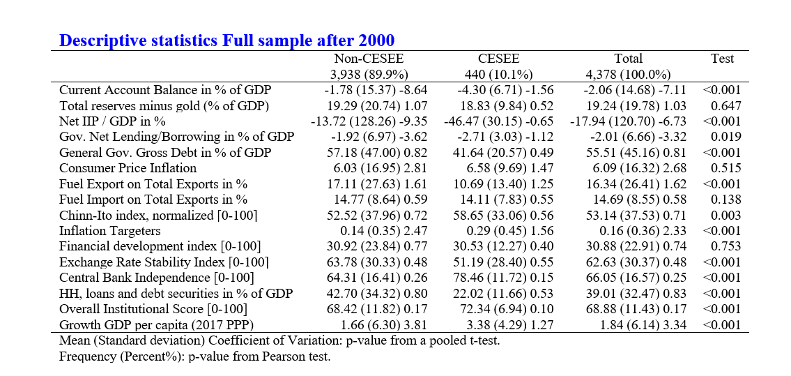
Let us start with the results that you will obtain after running a few lines of code directly in a Word file, for example:

The code is displayed below and produces a Word file with four “Tables 1” to have a deeper understanding of your data at the beginning of your research work:

putdocx begin, font("Times New Roman", 9)

local variables "CAB RESGDP NIIP GDeficit GDebt CPI FUELX FUELM ka_open IT FD ers cbie_index HH_LS inst gGDP_PKPPP"

dtable `variables' if period>2000, /*
  */ by(cesee, totals tests) /*
  */ column(by(hide)) /*
  */ sample(, place(seplabels)) /*
  */ title(Descriptive statistics /*
  */ Full sample after 2000) /*
  */ titlestyles(font(, size(12) color(blue) bold)) /*
  */ nformat(%6.0fc frequency) /*
  */ nformat(%6.2f  mean sd cv) /*
  */ continuous(, statistic(mean sd cv)) /*
  */ halign(right) /*
  */ note(Mean (Standard deviation) /*
  */ Coefficient of Variation: /*
  */ p-value from a pooled t-test.) /*
  */ note(Frequency (Percent%):/*
  */ p-value from Pearson test.) 

collect style putdocx, halign(center) /*
 */ layout(autofitcontents)

putdocx collect

dtable `variables' if period>2010, /*
  */ by(cesee, totals tests) /*
  */ column(by(hide)) /*
  */ sample(, place(seplabels)) /*
  */ title(Descriptive statistics Full sample after 2010) /*
  */ titlestyles(font(, size(12) color(blue) bold)) /*
  */ nformat(%6.0fc frequency) /*
  */ nformat(%6.2f  mean sd cv) /*
  */ continuous(, statistic(mean sd cv)) /*
  */ halign(right) /*
  */ note(Mean (Standard deviation) Coefficient of Variation: /*
  */ p-value from a pooled t-test.) /*
  */ note(Frequency (Percent%): p-value from Pearson test.)  
 
collect style putdocx, halign(center) /*
 */ layout(autofitcontents)

putdocx collect

putdocx pagebreak

dtable `variables' if period>2000, /*
  */ by(ceseeinstQ4, totals tests) /*
  */ column(by(hide)) /*
  */ sample(, place(seplabels)) /*
  */ title(Descriptive statistics Full sample after 2000) /*
  */ titlestyles(font(, size(12) color(blue) bold)) /*
  */ nformat(%6.0fc frequency) /*
  */ nformat(%6.2f  mean sd cv) /*
  */ continuous(, statistic(mean sd cv)) /*
  */ halign(right) /*
  */ note(Mean (Standard deviation) Coefficient of Variation: /*
  */ p-value from a pooled t-test.) /*
  */ note(Frequency (Percent%): p-value from Pearson test.)  
 
collect style putdocx, halign(center) /*
 */ layout(autofitcontents)

putdocx collect
 
dtable `variables' if period>2010, /*
  */ by(ceseeinstQ4, totals tests) /*
  */ column(by(hide)) /*
  */ sample(, place(seplabels)) /*
  */ title(Descriptive statistics Full sample after 2010) /*
  */ titlestyles(font(, size(12) color(blue) bold)) /*
  */ nformat(%6.0fc frequency) /*
  */ nformat(%6.2f  mean sd cv) /*
  */ continuous(, statistic(mean sd cv)) /*
  */ halign(right) /*
  */ note(Mean (Standard deviation) Coefficient of Variation: /*
  */ p-value from a pooled t-test.) /*
  */ note(Frequency (Percent%): p-value from Pearson test.) 

collect style putdocx, halign(center) /*
 */ layout(autofitcontents)
 
putdocx collect
 
putdocx save ds_cesee_29july.docx, replace

Let us focus on a specific part of the code and explain the role of the different options:

putdocx begin, font("Times New Roman", 9)

local variables "CAB RESGDP NIIP GDeficit GDebt CPI FUELX FUELM ka_open IT FD ers cbie_index HH_LS inst gGDP_PKPPP"

dtable `variables' if period>2000, /*
  */ by(cesee, totals tests) /*
  */ column(by(hide)) /*
  */ sample(, place(seplabels)) /*
  */ title(Descriptive statistics Full sample after 2000) /*
  */ titlestyles(font(, size(12) color(blue) bold)) /*
  */ nformat(%6.0fc frequency) /*
  */ nformat(%6.2f  mean sd cv) /*
  */ continuous(, statistic(mean sd cv)) /*
  */ halign(right) /*
  */ note(Mean (Standard deviation) Coefficient of Variation: /*
  */ p-value from a pooled t-test.) /*
  */ note(Frequency (Percent%): p-value from Pearson test.) 

collect style putdocx, halign(center) /*
 */ layout(autofitcontents)

putdocx collect

putdocx save ds_cesee_29july.docx, replace

After opening a Word file with ‘putdocx begin’, you can choose the font and the size with the ‘font’ option, we can start with ‘dtable’ that is the name of the main command, besides the variables that stored in a local variable named ‘variable’ (thus, you need to run the subsequent commands with the local command).

Then, come the options. The ‘by’ option allows selecting the group that you want to distinguish and the ‘totals’ and ‘test’ sub-options allow displaying the totals and t-tests for difference in the means throughout the table. The ‘column’ option allows you to hide the ‘by’ column in the Table, as it may be considered redundant.

The ‘title’ and ‘titlestyles’ options control the title. You can control the font size and the color with the sub-options ‘size’ and ‘color’. The ‘nformat’ options control the format of the numbers in the Table. For example, %6.0fc will display a maximum of 6 numbers and 0 decimal. The ‘fc’ part is adapted for large number like frequencies. In the case of the statistics, mean, standard deviation and coefficient of variation ‘%6.0f’ is adapted, as these values are usually small. If you want to add additional statistics in the Table, you may need to add the ‘continuous’ option. Finally, you can add notes with the ‘note’ option, and choose the alignment for the Table with ‘halign’. Under the Table, the ‘note’ option allows including some notes to ease the reading of the Table.

Before closing and saving the Word file, you can customize the Table placement and layout with ‘collect style putdocx’ and the options ‘halign’ and ‘layout’. Then, you need to collect the Table with ‘putdocx collect’. Finally, you can save the Word file with ‘putdocx save’.

More on dtable in the Stata Base Reference Manual.