Graph combine and loops with STATA

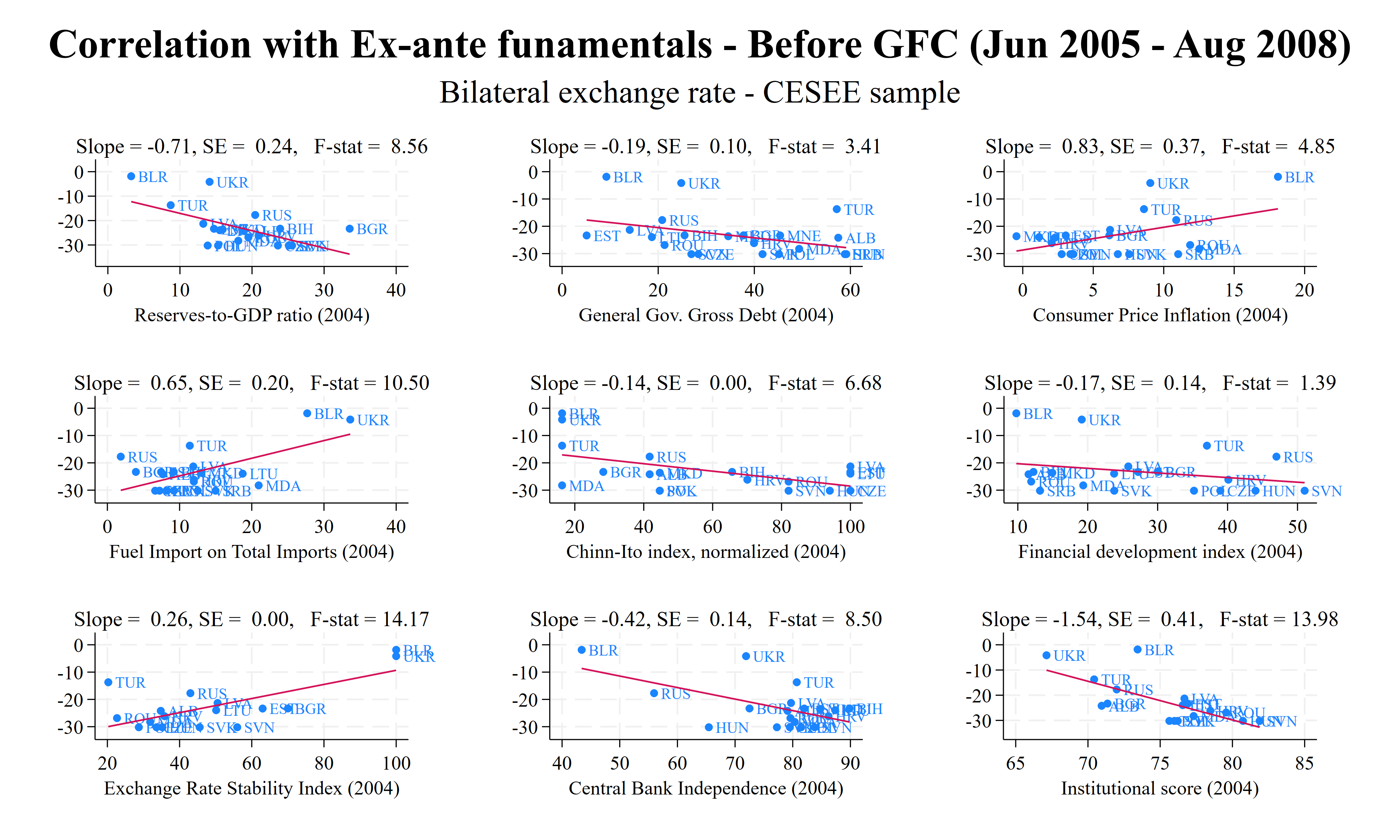
In this blog, I will show how to use the Stata commands ‘graph combine’ and ‘foreach loop’ to produce high-quality graphs that may be included in the Data section of your paper, together with the “Table 1”, see this blog on Descriptive Statistics for more details and codes. We are going to reproduce the figure below, that reports the scatter plots and regressions lines for nine OLS univariate regressions between the bilateral exchange rate and ex-ante fundamentals, along with the slopes, standards errors (SE), and Fisher statistics. Special thanks go to Blaise Gnimassoun for showing me this trick in our joint publication in Emerging Markets Review.

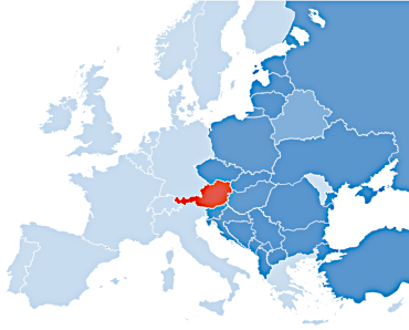
Let me give you a bit of context for this blog. For an ongoing research project, I currently explore the importance of fundamentals observed one year before ECB’s monetary cycles for several variables like bilateral exchange rates, long-term interest rates, stock prices, inflation, real GDP growth, and real GDP growth’s coefficient of variation in the CESEE regions. The CESEE region’s relevance and composition are described on the websites of both the Oesterreichische Nationalbank (OeNB) and the International Monetary Fund.

This project is the extension of an ADB project on the resilience of emerging markets during US monetary cycles (also available as a NBER WP). This project has been covered on a previous blog of mine. In this ongoing project, we focus on the impact of the ECB’s monetary cycles on the CESEE countries. Stay tuned, more to come on this in the following months. Let us dive into the STATA code now. As a first step, I report the full code below. In the following parts of the blogs, I will explain each part of the code.

lab var RESGDP "Reserves-to-GDP ratio (2004)" 
lab var GDebt "General Gov. Gross Debt (2004)" 
lab var CPI "Consumer Price Inflation (2004)"
lab var FUELM "Fuel Import on Total Imports (2004)"
lab var ka_open "Chinn-Ito index, normalized (2004)"
lab var FD "Financial development index (2004)"
lab var ers "Exchange Rate Stability Index (2004)"
lab var cbie_index "Central Bank Independence (2004)"
lab var inst "Institutional score (2004)"

**# Cycle 1

**
local graphs " "
// Run everything between preserve and restore
preserve
keep if cesee==1 & time==1
# delimit ;
local variables "RESGDP GDebt 
CPI FUELM ka_open FD ers 
cbie_index inst"; 
foreach v in `variables'{ ;
reg DXRcycle_1_w05 `v' if cesee==1;
mat b=e(b);
mat v=e(V);
local a:di %5.2f b[1,1];
local se_a:di %5.2f v[1,1];
local se_a_: di %5.2f sqrt(`se_a');
local F:di %5.2f e(F);
twoway (scatter DXRcycle_1_w05 `v' if cesee==1, 
mlabel(imfcode) mlabsize(small)) 
(lfit DXRcycle_1_w05 `v' if cesee==1), 
legend(off) name(`v'XR1, replace) 
graphregion(margin(l+2 r+8)) 
subtitle("Slope = `a', SE = `se_a_',  
F-stat = `F'") ;
local graphs "`graphs' `v'XR1" ;
};
# delimit cr
restore
**

# delimit ;
graph combine `graphs', title("{bf:Correlation with
Ex-ante funamentals - Before GFC (Jun 2005 - Aug 2008)}")
subtitle("Bilateral exchange rate - CESEE sample");
graph close `graphs';
# delimit cr

# delimit ;
graph rename XR_Funda_cycle1, replace ;
graph export XR_Funda_cycle1.png, as(png)
 width(4000) replace ;
graph export XR_Funda_cycle1.pdf, as(pdf)
 replace ;
graph export XR_Funda_cycle1.svg, as(svg)
 replace ;
#delimit cr

The first part of the code is not very interesting as it consists in labeling the variables. Do not forget to run everything between ‘preserve’ and ‘restore’ to keep your dataset intact. In the loop, I use the pound delimiter ;, which has been covered in this blog. After the regression, I use “mat b=e(b)” and “mat v=e(V)” to store the results of each estimate in matrices. The first matrix stores the coefficients and the second matrix is the variance-covariance matrix. I store the slope, the SE, and the F-stat with the local command. Then, I use the ‘subtitle’ option to include all these pieces of information in each graph. Less importantly, I removed the legend and customized the margins.

foreach v in `variables'{ ;
reg DXRcycle_1_w05 `v' if cesee==1;
mat b=e(b);
mat v=e(V);
local a:di %5.2f b[1,1];
local se_a:di %5.2f v[1,1];
local se_a_: di %5.2f sqrt(`se_a');
local F:di %5.2f e(F);
twoway (scatter DXRcycle_1_w05 `v' if cesee==1, 
mlabel(imfcode) mlabsize(small)) 
(lfit DXRcycle_1_w05 `v' if cesee==1), 
legend(off) name(`v'XR1, replace) 
graphregion(margin(l+2 r+8)) 
subtitle("Slope = `a', SE = `se_a_',  
F-stat = `F'") ;
local graphs "`graphs' `v'XR1" ;
};

Inspired by this discussion on the Stata Forum (especially the Friedrich Huebler‘s comments), I decided to include a new ‘local’ variable in the ‘graph combine’ part of the graph to make it more efficient and not waste time in reporting the name of each graph. Do not forget to add local graphs " " at the beginning of the code.

# delimit ;
graph combine `graphs', title("{bf:Correlation with
Ex-ante funamentals - Before GFC (Jun 2005 - Aug 2008)}")
subtitle("Bilateral exchange rate - CESEE sample");
graph close `graphs';
# delimit cr

Finally, you can save the graphs in three different formats, two of them are in vectorial format PDF and SVG. I use personally PNG with Word, PDF with LaTeX, and SVG on websites.

# delimit ;
graph rename XR_Funda_cycle1, replace ;
graph export XR_Funda_cycle1.png, as(png)
 width(4000) replace ;
graph export XR_Funda_cycle1.pdf, as(pdf)
 replace ;
graph export XR_Funda_cycle1.svg, as(svg)
 replace ;
#delimit cr