Estima, the company that develops and sells the RATS software, has released a new version of their online help. Notably, they incorporated the user guide version of the chapter on VAR. The online chapter is a good balance between theory and application. We are going to use the data covered in this publication, that relates oil price dynamics to the political tensions between the US and China in order to illustrate the commands to get the impulse response functions (IRF), historical decompositions (HD), and variance decompositions (VD). Let me remind that I already covered similar commands in the following two blogs: “Local Projection with Stata” and “Moving Block Bootstrap with GAUSS” using a similar dataset. The full code is available on my GitHub. Special thanks go to Francisco Serranito for his RATS lectures during my Master’s thesis.
I start with the impulse response functions using Monte Carlo Integration for the confidence bands, please refer to this part of the help for more details. I will import the data and make the necessary transformation for the variables.
OPEN DATA "C:\Users\jamel\Dropbox\Latex\PROJECTS\23-05-geopolitical-risk-pol-tension-oil-price\Data and command\lpirf_PRI_GPR.dta"
CALENDAR(M) 1960:1
DATA(FORMAT=DTA,RIGHT=9) 1960:01 2019:12 PERIOD PRI PRI_S PRO RPO DEM DINV GPRCN IGREA

set lpri = PRI_S
set lpro = 1*log(PRO)
set lrpo = 1*log(RPO)
set ldem = 1*log(DEM)
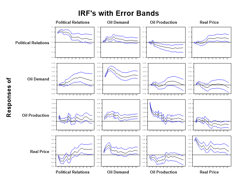
Now, I have to specify the VAR system with the appropriate number of lags and steps for the visualization of the IRF. With the @montevar procedure, I will compute the confidence bands for the VAR. In the help, they mention that “The shocks are in the columns and the response variables are in the rows.”
*****************************************************************

compute  nlags  = 24
compute  nsteps = 48

system(model=prirpo)
variables lpri ldem lpro lrpo
lags 1 to nlags
det constant
end(system)

compute implabel=|| $
  "Political Relations",$
  "Oil Demand",$
  "Oil Production",$
  "Real Price"||

estimate(noprint) 1989:01 2019:12

@montevar(draws=4000,model=prirpo,$
   shocks=implabel,varlabels=implabel$
   header="IRF's with Error Bands")
In the first column, we can observe the effect of an identified shock of political relations between the US and China on the oil market, for more detail, please consult this article.
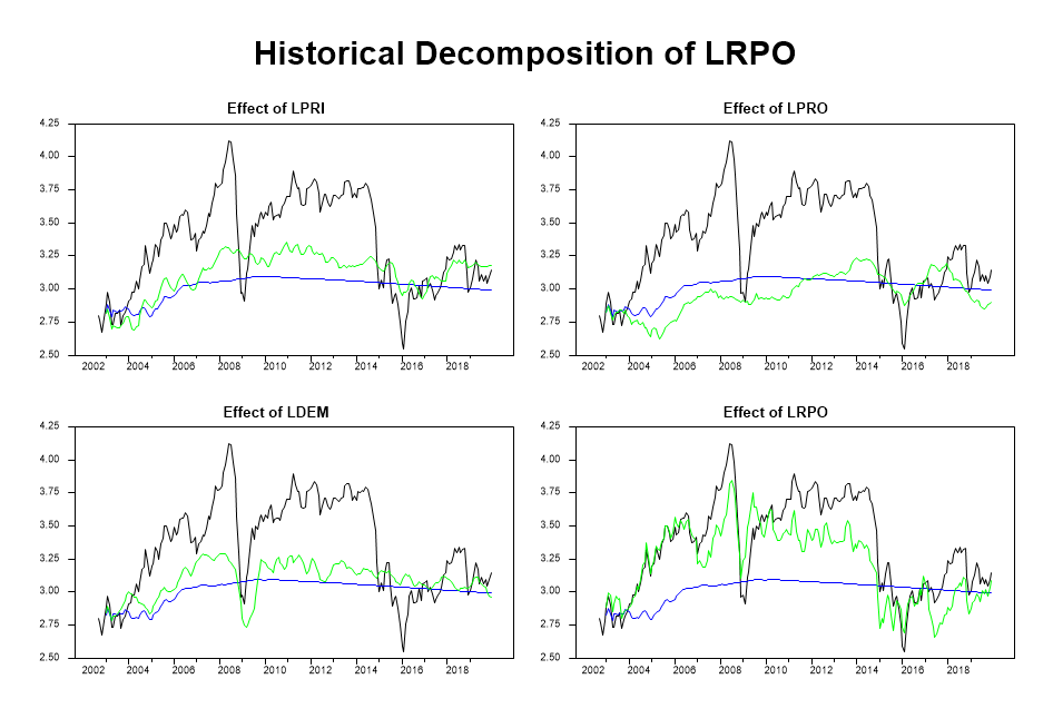
We can turn now to the HD. First, I have to include the forecast horizon. In this example, I will choose a forecasting period from January 2003 to December 2019. Then, I declare the variable labels and include some code that will be helpful in the loop to produce the graphs. The HD are computed using the @history function. The loop allows computing HD for each variable. Let us focus on the real price of oil in log. They mention that “With this color scheme, the black line is the actual data, the blue is the base forecast (which starts a year into the graph) and the green is the base forecast plus the effects of the shock”.
compute hstart = 2003:1
compute hend   = 2019:12

compute varlabels=|| $
  "Real Price",$
  "Oil Production",$
  "Oil Demand",$
"Political Relations"||

compute neqn=%modelsize(prirpo)
dec vect[int] depvar(neqn)
dec vect[string] varlabels(neqn) shocklabels(neqn)
ewise varlabels(i)=%modellabel(prirpo,i)
ewise shocklabels(i)=%modellabel(prirpo,i)
compute depvar=%modeldepvars(prirpo)

estimate(noprint,noftests,resids=resids) 1989:01 2019:12

HISTORY(MODEL=PRIRPO,add,base=base,effects=effects,FROM=2003:01,TO=2019:12,PRINT)

compute rows=fix(sqrt(neqn))
compute cols=(neqn-1)/rows+1
do i=1,neqn
   spgraph(vfields=rows,hfields=cols,window=varlabels(i),$
     header="Historical Decomposition of "+varlabels(i))
   do j=1,neqn
      *
      * This graphs the actual data (including four pre-sample values),
      * the base forecast, and the effects of shock J on variable I.
      *
      graph(header="Effect of "+shocklabels(j)) 3
      # depvar(i) hstart-4 hend
      # base(i)
      # effects(i,j)
   end do j
   spgraph(done)
end do i

We can observe that the political relations between the US and China contributed positively to oil prices during the GFC and the fall of commodity prices in 2016.
Let us conclude this blog with the VD. I will use the ERROR instruction over 48 months to capture the long-lasting effect of political relations on the oil price.
*****************************************************************

system(model=prirpo)
variables lpri ldem lpro lrpo
lags 1 to 24
det constant
end(system)
estimate(cvout=v,noprint) 1989:01 2019:12
*
*  The first decomposition is done in the original order:
*  system(model=prirpo)
*  lpri ldem lpro lrpo.
*
ERRORS(MODEL=PRIRPO,STEPS=48,PRINT)

*****************************************************************
We can observe that innovations on political relations explain 17.38% of the variance of the one-step forecast error for the oil prices at the horizon of 48 months.
Decomposition of Variance for Series LRPO
 Step   Std Error    LPRI     LDEM     LPRO    LRPO
      1 0.06569657    0.549    2.935    1.293  95.223
      2 0.10028101    1.410    4.898    1.468  92.224
      3 0.12768230    3.057    7.413    2.425  87.105
      4 0.14945727    5.311   10.216    3.003  81.470
      5 0.16610357    7.384   12.500    2.860  77.256
      6 0.18036029    8.421   14.910    2.987  73.682
      7 0.19271057    9.595   17.552    2.959  69.895
      8 0.20462953   10.483   20.109    3.092  66.316
      9 0.21439487   10.675   22.103    3.431  63.791
     10 0.22218547   10.490   23.357    4.187  61.965
     11 0.22842352   10.285   23.388    5.202  61.124
     12 0.23499869    9.801   22.763    6.757  60.679
     13 0.24118163    9.376   22.172    7.783  60.669
     14 0.24642067    9.303   21.808    8.508  60.381
     15 0.25172207    9.580   21.452    9.395  59.574
     16 0.25559427    9.859   21.144   10.115  58.882
     17 0.25950074   10.231   21.041   10.873  57.855
     18 0.26274478   10.216   21.055   11.452  57.277
     19 0.26530778   10.032   21.104   11.795  57.069
     20 0.26802469    9.849   20.868   12.350  56.933
     21 0.27151787    9.664   20.516   12.757  57.063
     22 0.27525937    9.485   20.151   12.962  57.402
     23 0.27941861    9.342   19.766   12.828  58.063
     24 0.28297700    9.420   19.490   12.545  58.545
     25 0.28583711    9.462   19.366   12.330  58.842
     26 0.28833113    9.472   19.265   12.164  59.100
     27 0.29036112    9.506   19.125   12.152  59.217
     28 0.29222649    9.560   18.991   12.152  59.296
     29 0.29414391    9.703   18.835   12.089  59.373
     30 0.29631012   10.069   18.629   11.969  59.333
     31 0.29877318   10.554   18.389   11.829  59.228
     32 0.30160973   11.176   18.106   11.672  59.047
     33 0.30467669   11.887   17.822   11.521  58.770
     34 0.30770065   12.573   17.623   11.379  58.425
     35 0.31047493   13.180   17.511   11.235  58.074
     36 0.31306040   13.638   17.476   11.126  57.760
     37 0.31569872   14.032   17.452   11.033  57.483
     38 0.31830341   14.435   17.448   10.933  57.184
     39 0.32107546   14.827   17.419   10.876  56.878
     40 0.32378098   15.148   17.363   10.855  56.634
     41 0.32645988   15.453   17.293   10.864  56.390
     42 0.32927545   15.712   17.279   10.916  56.092
     43 0.33206894   15.943   17.312   10.989  55.756
     44 0.33481253   16.232   17.355   11.083  55.330
     45 0.33743505   16.516   17.416   11.229  54.839
     46 0.33997976   16.801   17.491   11.433  54.276
     47 0.34247046   17.087   17.545   11.671  53.697
     48 0.34504562   17.385   17.551   11.940  53.124
1 Comment
[…] two blogs on SVAR with RATS and on SVAR with sign restrictions with Stata, allow me to introduce the estimation of SVAR with […]