In joint work with Marco Gallegati, William Ginn, Solomos Solomou, and Kun Tian—Climate Shocks in Global Oil Markets: Time-Varying ENSO Transmission to WTI Spot and Futures Prices—we study how phase-specific El Niño–Southern Oscillation (ENSO) shocks affect real WTI spot and futures prices.
A recurring problem in empirical macroeconomics is that the word correlation is sometimes used too broadly. A regression coefficient is not automatically causal. But the opposite mistake is also possible: structurally identified impulse responses may be described as correlations merely because the paper does not separately quantify every economic mechanism through which the shock reaches the outcome.
Those are different questions. The first concerns identification: is the variation in the shock exogenous, and is the contemporaneous ordering defensible? The second concerns transmission: through which demand, supply, financial, or expectations channels does the identified shock affect oil prices?
Main takeaway. ENSO is a physically external climate disturbance. At monthly frequency, it can be ordered first under a credible short-run restriction because innovations in oil prices, global oil production, world industrial production, and the exchange rate cannot contemporaneously generate tropical-Pacific sea-surface-temperature anomalies. The model also conditions on twelve months of ENSO, oil-price, world industrial production, global oil production, and exchange-rate histories. The resulting local-projection paths are therefore structural dynamic causal responses—not bivariate correlations. The additional responses of world industrial production, global oil production, and the nominal effective exchange rate provide evidence on the indirect channels through which the shock is transmitted.
1. What would an “interesting correlation” look like?
A simple correlational exercise might estimate
\[ op_t=\alpha+\beta ENSO_t+e_t, \]where \(op_t\) is an oil price and \(ENSO_t\) is a contemporaneous climate indicator.
Such an equation would leave the major identification and dynamics questions unresolved. It would not condition on oil-price persistence, global demand, global oil production, dollar movements, the persistence of the ENSO episode, or the history of the opposite ENSO phase. It would not specify why the climate variable can be treated as an exogenous shock, and it would not trace the adjustment of oil prices month by month.
That is not our empirical design.
We estimate horizon-specific responses of real WTI spot and futures prices to phase-specific absolute Niño 3.4 sea-surface-temperature anomalies. El Niño and La Niña are treated separately, and the dynamic effects are traced over horizons extending to two years. The shock variables are
\[ s_t^{EN}=|SST_t|\mathbf{1}\{EN_t=1\}, \qquad s_t^{LN}=|SST_t|\mathbf{1}\{LN_t=1\}, \]where \(SST_t\) is the Niño 3.4 anomaly measured in degrees Celsius.
The empirical question is therefore:
\[ \text{How does the path of oil prices change after an identified ENSO shock?} \]That is an impulse-response question, not a contemporaneous correlation exercise.
2. The shock is identified before its propagation is estimated
The central distinction is between identifying the shock and estimating its propagation. Identification answers: which contemporaneous movement can be interpreted as the ENSO shock? Propagation answers: how do oil prices and the other variables evolve during the months following that identified shock?
This distinction is essential because a local projection does not need to leave structural identification to a VAR. A short-run restriction can identify the shock directly in the LP specification. The LP then estimates one response coefficient for each horizon.
2.1. Start from a structural monthly system
Consider the monthly vector
\[ X_t= \begin{bmatrix} ENSO_t\\ WIP_t\\ GOP_t\\ NEER_t\\ OP_t \end{bmatrix}, \]where \(WIP_t\) denotes the monthly World Industrial Production index made available on Christiane Baumeister’s data website and associated with Baumeister and Hamilton (2019), \(GOP_t\) denotes global oil production, \(NEER_t\) is the U.S. nominal effective exchange rate, and \(OP_t\) is the real WTI spot or futures price. The WIP measure captures the level of global industrial activity rather than aggregate global GDP, making it especially relevant for oil demand because manufacturing, mining, utilities, freight, and other industrial activities are energy intensive.
A structural dynamic system can be written schematically as
\[ A_0X_t = A_1X_{t-1}+\cdots+A_{12}X_{t-12} +\varepsilon_t, \]where \(A_0\) describes the contemporaneous relations among the variables and \(\varepsilon_t\) contains economically interpretable structural shocks. The purpose of a short-run restriction is to place economically defensible zero restrictions on \(A_0\), or equivalently on its inverse, so that the structural shock can be recovered.
Under a recursive ordering with ENSO first, the contemporaneous impact representation is
\[ u_t=P\varepsilon_t, \]where \(u_t\) denotes the innovations after conditioning on the lagged system and \(P\) is lower triangular:
\[ P= \begin{bmatrix} p_{11} & 0 & 0 & 0 & 0\\ p_{21} & p_{22} & 0 & 0 & 0\\ p_{31} & p_{32} & p_{33} & 0 & 0\\ p_{41} & p_{42} & p_{43} & p_{44} & 0\\ p_{51} & p_{52} & p_{53} & p_{54} & p_{55} \end{bmatrix}. \]The first equation is therefore
\[ u_t^{ENSO}=p_{11}\varepsilon_t^{ENSO}, \]so that
\[ \varepsilon_t^{ENSO}=\frac{u_t^{ENSO}}{p_{11}}. \]This is the key result. Because ENSO is first, the first innovation contains no contemporaneous shock to world industrial production, global oil production, the exchange rate, or oil prices. It is proportional only to the structural ENSO shock. The expression “up to normalization” simply means that the shock can be scaled as a one-unit, one-degree-Celsius, or one-standard-deviation disturbance without changing its economic identity.
2.2. A simple two-variable example
The logic is easiest to see in a two-variable system containing ENSO and the oil price:
\[ ENSO_t = \Pi_1\mathcal I_{t-1} +\varepsilon_t^{ENSO}, \] \[ OP_t = \lambda ENSO_t +\Pi_2\mathcal I_{t-1} +\varepsilon_t^{OP}. \]The first equation says that current ENSO is determined by its lagged information and by the current structural ENSO shock. Current oil-price innovations do not enter that equation. The second equation allows the oil price to react immediately to the current ENSO shock through \(\lambda\). Thus, the ordering does not rule out a contemporaneous effect of ENSO on oil prices. It rules out only the physically implausible reverse effect of a current oil-market shock on current tropical-Pacific SST conditions.
The same logic extends to world industrial production, global oil production, and the NEER. All variables placed after ENSO may react within month \(t\). None of their current structural shocks is allowed to generate the ENSO shock within that same month.
2.3. Identification and propagation are separate steps
Once \(\varepsilon_t^{ENSO}\) has been identified, one can estimate its effect on an outcome at horizon \(h\):
\[ y_{t+h} = \alpha_h +\theta_h\varepsilon_t^{ENSO} +\Gamma_h’\mathcal I_{t-1} +e_{t+h}. \]The short-run restriction determines the meaning of \(\varepsilon_t^{ENSO}\). The local projection determines the sequence
\[ \theta_0,\theta_1,\ldots,\theta_{24}, \]which traces the impact response and the subsequent monthly propagation. A VAR would propagate the same identified shock by iterating a fitted dynamic system. A local projection estimates each horizon directly. The estimator changes; the structural meaning of the identified first-ordered shock does not.
“Short-run restriction” therefore does not mean that the effect must be short-lived. The restriction concerns only the contemporaneous causal ordering at date \(t\). The resulting structural response may persist for many months or years.
A companion EconMacro post develops this point in more detail: Can Local Projections Have Short-Run Restrictions?
3. Why ordering ENSO first is credible at monthly frequency
No recursive ordering is assumption-free. The correct question is not whether a restriction exists, but whether the restriction is economically, physically, and temporally defensible.
3.1. What the ENSO-first restriction says
Ordering ENSO first imposes the following contemporaneous exclusions:
\[ \frac{\partial ENSO_t}{\partial\varepsilon_t^{OP}} = \frac{\partial ENSO_t}{\partial\varepsilon_t^{WIP}} = \frac{\partial ENSO_t}{\partial\varepsilon_t^{GOP}} = \frac{\partial ENSO_t}{\partial\varepsilon_t^{NEER}} =0. \]In words, current innovations in oil prices, world industrial production, global oil production, and the exchange rate do not alter the current ENSO shock within the same month.
The ordering simultaneously allows
\[ \frac{\partial OP_t}{\partial\varepsilon_t^{ENSO}}, \quad \frac{\partial WIP_t}{\partial\varepsilon_t^{ENSO}}, \quad \frac{\partial GOP_t}{\partial\varepsilon_t^{ENSO}}, \quad \frac{\partial NEER_t}{\partial\varepsilon_t^{ENSO}} \]to be nonzero. Hence, the economic variables may respond on impact to ENSO. The restriction is directional, not symmetric.
3.2. Why the reverse causal direction is implausible
For the ENSO–oil-price relationship, the contemporaneous exclusion is unusually clear:
\[ \text{monthly oil-market innovation} \not\rightarrow \text{contemporaneous Niño 3.4 SST anomaly}. \]A movement in WTI spot or futures prices cannot change the temperature of the tropical Pacific within the same month. Nor can an exchange-rate innovation, an unexpected monthly change in world industrial production, or an oil-production shock create an El Niño or La Niña episode on impact. ENSO originates from large-scale ocean–atmosphere dynamics whose physical evolution is independent of contemporaneous oil-market valuation.
The reverse direction is plausible. ENSO can alter temperatures, rainfall, storms, heating and cooling needs, transportation, refinery conditions, production, inventories, agricultural activity, expectations, and risk pricing. These responses may begin during the same month and continue over subsequent horizons.
If oil prices were ordered before ENSO, the recursive system would allow a current oil-price shock to move ENSO within the same month. That would be difficult to defend physically. The ENSO-first ordering is therefore not an arbitrary choice made to obtain a desired response; it follows from the direction of physical causation.
3.3. Why monthly frequency strengthens the restriction
The observation period matters for a short-run restriction. Here, “short run” means within the monthly observation interval. The maintained restriction is that economic and oil-market shocks do not feed back into Niño 3.4 SST conditions during that month.
This assumption is particularly credible because the economic variables are financial or macroeconomic outcomes, whereas ENSO is a large-scale physical ocean–atmosphere phenomenon. Even though ENSO develops over time and may be forecast, predictability does not imply that the oil market causes it. Forecasts may change when traders respond, but they do not reverse the physical causal ordering.
3.4. What the restriction does not claim
The ENSO-first restriction does not claim that:
- ENSO is completely unpredictable from climate information;
- oil prices cannot react during month \(t\);
- world industrial production, global oil production, or exchange rates are unaffected on impact;
- the ENSO effect disappears after one month;
- all transmission mechanisms are known in advance.
It claims only that the structural innovations in the later-ordered economic variables do not contemporaneously cause the first-ordered ENSO shock. That narrow restriction is sufficient to identify the first structural shock in the recursive system.
The physical origin of ENSO therefore supports the short-run restriction independently of the observed oil-price response. This is also consistent with the climate–macroeconomics literature, which treats ENSO as externally generated climate variation when estimating its effects on output, inflation, energy prices, and other commodity prices.
4. The model conditions on the standard determinants of global oil prices
The contemporaneous ordering is reinforced by a rich monthly information set. The projections condition on twelve lags of:
- the phase-specific ENSO shock;
- the opposite ENSO phase;
- the WTI spot or futures price;
- world industrial production;
- global crude-oil production;
- the U.S. nominal effective exchange rate.
World industrial production is measured by the monthly World Industrial Production index obtained from Christiane Baumeister’s website and associated with Baumeister and Hamilton (2019). In the Stata files, its log is denoted by LGECON. This is not a generic global-GDP or service-sector indicator. It is a monthly measure of the scale of global industrial production, which is particularly suitable for an oil-market application because industrial activity is a major source of petroleum demand.
Schematically, the El Niño projection is
\[ \begin{aligned} op_{t+h}^{WTI,x} =&\;\alpha_h +\theta_h^{EN}s_t^{EN} +\sum_{j=1}^{12}\rho_{j,h}^{EN}s_{t-j}^{EN}\\ &+\sum_{j=1}^{12}\delta_{j,h}^{LN}s_{t-j}^{LN} +\sum_{j=1}^{12}\Gamma_{j,h}’Z_{t-j} +e_{t+h}, \end{aligned} \]where
\[ Z_t= \left\{ op_t^{WTI,x}, WIP_t, GOP_t, NEER_t \right\}. \]The La Niña specification is symmetric.
Because LGECON is the log of the monthly WIP index and no growth transformation is applied, its impulse response is a log-level response. It measures the percentage displacement of the level of world industrial production from its no-shock path at each horizon. This is different from a monthly growth-rate response, which can turn positive during a recovery even while the level of industrial production remains below its counterfactual path. For the oil-demand channel, the log-level response is the more directly relevant object because it measures the scale of energy-intensive industrial activity.
The twelve ENSO lags are especially important because ENSO episodes are persistent. They prevent the coefficient on the current anomaly from merely reproducing the effects of a climate episode that began several months earlier. The model also conditions on the main determinants emphasized in the global oil-market literature: past oil prices, world industrial production as a measure of energy-intensive global demand, global oil production, and dollar valuation.
4.1. How the short-run ordering appears inside the local projection
The recursive short-run restriction is implemented directly through the timing of the regressors. The phase-specific ENSO shock enters at date \(t\), whereas the response variable and all economic variables ordered after ENSO begin at \(t-1\). The generic horizon-\(h\) equation is
\[ y_{t+h} = \alpha_h +\theta_h^p s_t^p +\Lambda_h’\mathcal I_{t-1} +e_{t+h}, \]where \(s_t^p\) is the current El Niño or La Niña shock and \(\mathcal I_{t-1}\) contains the twelve-month lag history of the ENSO variables, the response, oil prices, world industrial production, global oil production, and the NEER.
The timing can be read very literally:
- At \(t\): the identified ENSO shock is allowed to occur.
- Also at \(t\): the response variable may react to that shock; this is the horizon-zero effect \(\theta_0^p\).
- From \(t-1\) backward: the model conditions on the pre-shock history of the entire system.
- Not included at \(t\): contemporaneous oil prices, world industrial production, global oil production, and the NEER are not used as controls because they are permitted to respond immediately to ENSO.
This is the local-projection counterpart of placing ENSO first in a Cholesky ordering. For a first-ordered shock, there is no contemporaneous variable before the shock that must be partialled out. The shock is identified from its innovation relative to the lagged information set.
4.2. Why the controls must begin at \(t-1\)
Suppose the ENSO shock affects oil production or world industrial production within month \(t\). If one were to include \(GOP_t\) or \(WIP_t\) as contemporaneous controls in the oil-price projection, one would be conditioning on variables that may already have responded to the shock. This would block part of the impact transmission and change the estimand.
The same issue applies to the spot price, futures price, and NEER. These variables are potential outcomes or transmission variables, not predetermined confounders at date \(t\). Their histories belong in the conditioning set; their contemporaneous realizations do not belong there when ENSO is ordered first.
This is why the distinction between \(t\) and \(t-1\) is the identifying restriction:
\[ \boxed{ \text{ENSO shock at }t \quad+\quad \text{economic controls beginning at }t-1 } \]The restriction allows the causal effect to operate at horizon zero and at all later horizons while ruling out contemporaneous reverse causality into ENSO.
4.3. The role of lag conditioning
Because the model includes twelve lags, the current shock coefficient is not based on the raw level of ENSO alone. By the Frisch–Waugh–Lovell theorem, it is identified from the component of current ENSO intensity that remains after conditioning on the preceding system history:
\[ \widetilde s_t^p = s_t^p – \operatorname{Proj} \left( s_t^p\mid\mathcal I_{t-1} \right). \]For a first-ordered variable, this residualized current movement is the first equation’s innovation. Under the recursive normalization, it is proportional to the structural ENSO shock. The twelve lags therefore address persistence and pre-existing dynamics; the contemporaneous ordering gives the innovation its structural interpretation.
If the shock were ordered second rather than first, the LP would need to include the first-ordered variable contemporaneously. For example, if variable \(A_t\) were first and variable \(B_t\) second, the structural response to the second shock would be estimated from a projection containing both \(B_t\) and contemporaneous \(A_t\). The current value of \(A_t\) would orthogonalize the second shock. No such contemporaneous control is required for ENSO because nothing precedes it in the ordering.
4.4. Stata implementation
In Stata, the short-run restriction is implemented as follows:
locproj LO, ///
    shock(SSTEN) ///
    ylags(12) ///
    slags(12) ///
    controls(L(1/12).(LGECON LPROD LNEER SSTLN)) ///
    hor(0/24) ///
    vce(r) stats ///
    conf(90 95)
The options correspond directly to the identification argument:
shock(SSTEN)places the current El Niño shock at date \(t\).slags(12)conditions on the previous twelve months of the El Niño process.ylags(12)conditions on the previous twelve months of the response variable.controls(L(1/12).(...))includes twelve lags ofLGECON(the log WIP index), oil production, the NEER, and the opposite ENSO phase—but no contemporaneous values.hor(0/24)estimates the impact response and the subsequent responses through month 24.
The symmetric La Niña specification replaces SSTEN with SSTLN and places the twelve-month history of El Niño among the lagged controls.
This is a short-run-restricted local projection with a structurally identified climate shock and a substantial conditioning set. It allows the economic variables to react contemporaneously to ENSO, rules out contemporaneous feedback into ENSO, and traces the resulting causal path horizon by horizon. It is not a bivariate association between two contemporaneous series.
5. Local projections estimate the structural causal path
Once the ENSO shock has been identified, the local projection estimates, for every horizon \(h\),
\[ op_{t+h}^{WTI,x} = \alpha_h + \theta_h^p\varepsilon_t^{ENSO,p} + \Gamma_h’\mathcal I_{t-1} + v_{t+h,h}, \qquad p\in\{EN,LN\}. \]The sequence
\[ \theta_0^p,\theta_1^p,\ldots,\theta_{24}^p \]is the structural dynamic response of the oil price to the ENSO shock. Local projections estimate this response directly at each horizon rather than iterating a fitted transition matrix.
The time-varying extension allows the response to depend on calendar time:
\[ op_{t+h}^{WTI,x} = \alpha_{h,t} + \theta_{h,t}^p\varepsilon_t^{ENSO,p} + \Gamma_{h,t}’\mathcal I_{t-1} + v_{t+h}. \]Here \(h\) is the number of months after the shock, while \(t\) is the historical date at which the shock occurs. The shock remains structurally identified; what changes over time is the oil-market environment through which it propagates.
6. Direct oil-market pricing versus indirect transmission
The distinction between the direct oil-market pricing channel and the indirect economic channels is central to interpreting the results.
6.1 The direct oil-market pricing channel
An ENSO shock changes the information set of oil traders, producers, refiners, storage operators, and hedgers. It changes beliefs about future weather-sensitive demand, production disruptions, transportation conditions, inventories, and market tightness. These beliefs can be incorporated into oil prices before the underlying physical and macroeconomic effects are fully realized.
For a futures contract with maturity \(k\), a useful schematic representation is
\[ F_t^{(k)} = E_t(S_{t+k}) + RP_t^{(k)}, \]where \(F_t^{(k)}\) is the futures price, \(E_t(S_{t+k})\) is the expected future spot price, and \(RP_t^{(k)}\) is the futures risk premium. An ENSO shock can affect the current futures price through either component:
\[ \frac{\partial F_t^{(k)}}{\partial\varepsilon_t^{ENSO}} = \frac{\partial E_t(S_{t+k})}{\partial\varepsilon_t^{ENSO}} + \frac{\partial RP_t^{(k)}}{\partial\varepsilon_t^{ENSO}}. \]If El Niño is expected to reduce future heating-related demand or relax future market tightness, the expected future spot price may decline. If La Niña signals stronger weather-sensitive demand or greater disruption risk, expected future scarcity and the compensation required for bearing oil-market risk may increase.
The spot price can also adjust through decisions made inside the oil market. Expected future scarcity changes current inventory demand, storage incentives, refinery scheduling, hedging positions, and cash–futures arbitrage:
\[ \varepsilon_t^{ENSO} \rightarrow \text{expectations, inventories, storage, and hedging} \rightarrow S_t. \]This is called a direct oil-market pricing channel because the shock is incorporated into current spot and futures valuations without requiring a prior observed change in world industrial production, global oil production, or the exchange rate.
“Direct” does not mean “only at horizon zero.” Market participants may update the implications of an evolving ENSO episode over several months. Seasonal demand, production risks, and transport disruptions may become clearer gradually. A delayed medium-horizon price response is therefore fully consistent with direct market repricing.
6.2 The indirect economic channels
ENSO may also affect oil prices through intermediate economic variables:
\[ \varepsilon_t^{ENSO} \rightarrow WIP_{t+j} \rightarrow OP_{t+h}, \] \[ \varepsilon_t^{ENSO} \rightarrow GOP_{t+j} \rightarrow OP_{t+h}, \] \[ \varepsilon_t^{ENSO} \rightarrow NEER_{t+j} \rightarrow OP_{t+h}. \]The WIP response informs the industrial-demand channel: an ENSO shock changes the level of global industrial production, which changes energy-intensive demand for petroleum. The global-oil-production response informs the physical supply channel, while the NEER response informs the dollar-pricing channel.
Other potential intermediates not yet shown in these figures include physical inventories, refinery utilization, shipping costs, heating-degree days, and the slope of the oil futures curve.
6.3 What the oil-price impulse response contains
The estimated oil-price response is
\[ \theta_h^p = \frac{\partial op_{t+h}^{WTI,x}} {\partial\varepsilon_t^{ENSO,p}}. \]It is the structural causal response of the oil price to the ENSO shock. It incorporates all paths that operate after the shock, including direct oil-market repricing and indirect transmission through real and financial variables.
Conceptually, one may write
\[ \text{overall oil-price response} = \text{direct oil-market pricing} + \text{indirect economic transmission}. \]This expression is an economic interpretation, not a numerical mediation decomposition. The additional impulse responses show whether the proposed intermediate variables move in directions consistent with the price response. They do not mechanically assign a percentage of the oil-price effect to each channel. A formal mediation decomposition would require additional assumptions and a different empirical exercise.
7. What the new channel results show
The figures below report structural responses to one-degree phase-specific ENSO shocks. The solid line is the estimated response and the shaded region is the 95 percent confidence interval. Because oil prices, world industrial production, global oil production, and the NEER are expressed in logs, a coefficient of \(0.02\) is approximately a 2 percent response to a one-degree shock. For a sample-mean phase-specific shock, the response is correspondingly smaller: multiplying by approximately \(0.33\) for El Niño or \(0.39\) for La Niña provides a representative scaling.
7.1 El Niño: lower oil prices, weaker world industrial production, and an early supply expansion
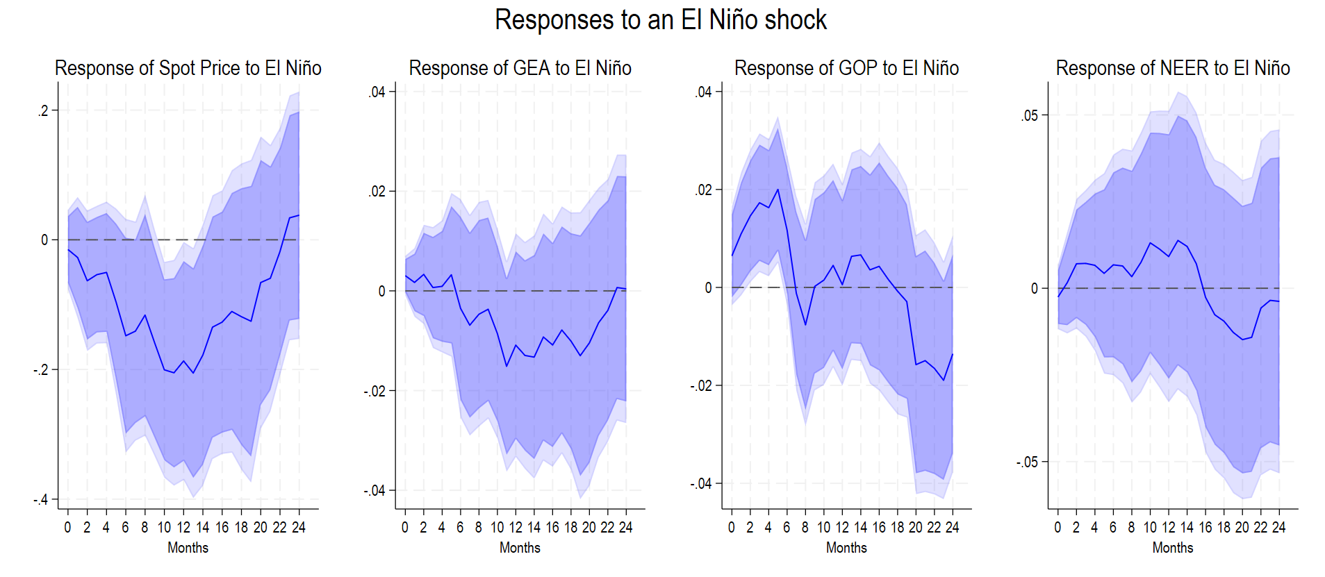
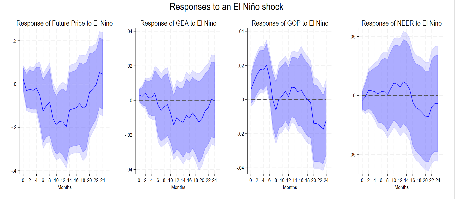
Oil spot and futures prices
The direct price response is clearly negative at medium horizons. Both spot and futures prices decline progressively, reaching a trough of roughly \(-0.20\) log points around months 10–13 before recovering toward zero. Over a substantial part of this medium-horizon interval, the 95 percent confidence band lies below zero.
The similarity between the spot and futures responses is informative. ENSO information is not confined to one segment of the market: it is reflected in both forward-looking contracts and the physical spot market. This is consistent with expectations, storage, inventory adjustment, and spot–futures arbitrage integrating the two markets. The figures do not by themselves establish that futures prices lead spot prices, but they show that the negative El Niño effect is broad-based.
World industrial production
The central estimate for the log level of world industrial production becomes negative after approximately five or six months, reaches its largest decline around months 11–14, and remains negative through much of the medium-horizon window. This timing overlaps with the period in which spot and futures prices are most negative.
The confidence interval frequently overlaps zero, so this result should be described as directionally coherent rather than uniformly precise. Economically, however, the sign and timing are consistent with an indirect industrial-demand channel. A lower level of world industrial production implies a smaller scale of energy-intensive manufacturing, mining, utilities, and freight activity, thereby weakening petroleum demand:
\[ \text{El Niño} \rightarrow \text{lower world industrial production} \rightarrow \text{weaker industrial oil demand} \rightarrow \text{lower oil prices}. \]Because this is a level response, a later improvement in monthly industrial-production growth would not necessarily overturn the result immediately: world industrial production could begin recovering while its level remains below the no-shock path.
Global oil production
Global oil production initially rises after the El Niño shock, with the positive response concentrated in approximately the first five months. A short-run supply expansion is consistent with downward pressure on oil prices. Production then becomes more volatile: it falls around months 7–9, returns to mildly positive territory at intermediate horizons, and declines again near the end of the response window.
The early production increase is the most economically useful part of this path for interpreting the price response:
\[ \text{El Niño} \rightarrow \text{initially higher oil supply} \rightarrow \text{lower oil prices}. \]The later oscillation indicates that production is not the sole channel and should not be used as a complete explanation of the persistent price decline.
Nominal effective exchange rate
The NEER response is small relative to the oil-price response and statistically imprecise. The central estimate is mildly positive at some earlier horizons and becomes negative after roughly month 16, but the 95 percent confidence interval generally includes zero.
This is an important null result. It suggests that the negative El Niño oil-price response is not primarily a dollar-valuation phenomenon. The evidence points more strongly toward direct oil-market repricing and real-side demand and supply channels.
El Niño synthesis
The timing suggests a combination of channels. Oil production rises early, potentially easing physical market tightness. World industrial production weakens later, reducing energy-intensive industrial oil demand. At the same time, spot and futures prices respond much more strongly than either intermediate variable, which is consistent with a direct pricing channel in which markets capitalize expected future conditions before they are fully realized.
\[ \begin{aligned} \text{El Niño} \rightarrow \begin{cases} \text{direct repricing of expected oil-market conditions},\\ \text{initial supply expansion},\\ \text{subsequent decline in world industrial production} \end{cases} \rightarrow \text{lower spot and futures prices}. \end{aligned} \]7.2 La Niña: higher oil prices, stronger world industrial production, and an early supply contraction
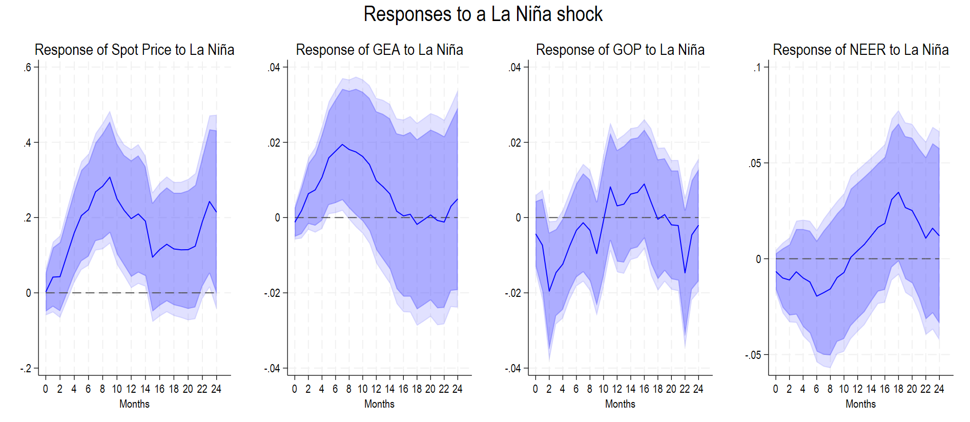
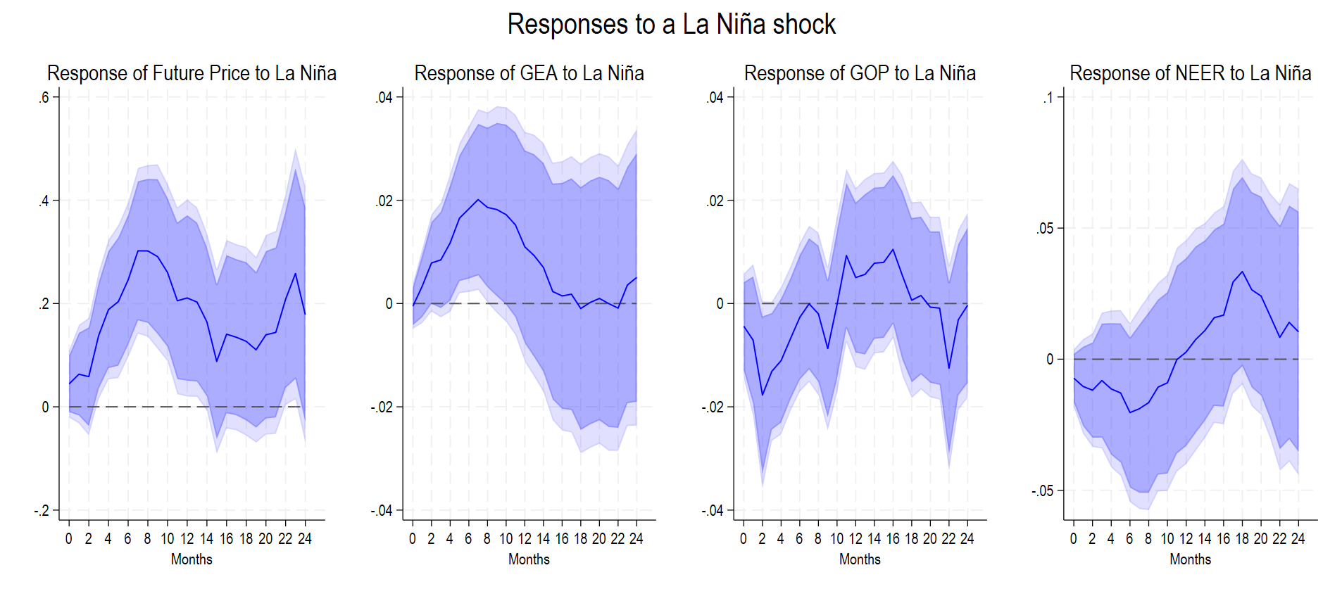
Oil spot and futures prices
The La Niña price response is positive, large, and more precisely estimated than most of the intermediate-variable responses. Spot and futures prices increase from the early horizons, peak at approximately \(0.30\) log points around months 8–9, and remain positive through much of the 4–14 month interval.
The confidence bands exclude zero over an economically important medium-horizon range. This is the clearest manifestation of the phase asymmetry: La Niña is an inflationary oil-market shock, whereas El Niño is deflationary.
Again, the spot and futures paths are extremely similar. The result is therefore not driven by a single price concept. Climate information appears to be incorporated throughout the integrated oil market.
World industrial production
The log level of world industrial production rises after a La Niña shock. The response strengthens over the first several months, reaches approximately \(0.02\) log points around months 7–9, and then gradually returns toward zero. The confidence band is above zero over part of the early-to-medium horizon.
This provides comparatively clear evidence for an indirect industrial-demand channel. A higher level of world industrial production means a larger scale of energy-intensive production and transport activity, which raises petroleum demand:
\[ \text{La Niña} \rightarrow \text{higher world industrial production} \rightarrow \text{stronger industrial oil demand} \rightarrow \text{higher oil prices}. \]The timing is particularly informative. The positive WIP response develops over the same interval in which the oil-price response becomes largest.
Global oil production
Global oil production initially falls, reaching a decline of roughly \(-0.02\) log points near month 2. This short-run supply contraction is consistent with the initial increase in oil prices. Production then oscillates around zero, becoming positive at some medium horizons before weakening again later.
The most defensible interpretation is therefore a short-run supply channel:
\[ \text{La Niña} \rightarrow \text{initially lower oil supply} \rightarrow \text{higher oil prices}. \]As in the El Niño case, the subsequent oscillation indicates that production alone does not explain the full persistence and size of the price response.
Nominal effective exchange rate
The NEER initially declines modestly and later becomes positive, but the confidence bands are wide and generally include zero. There is therefore little evidence that the dollar exchange-rate channel is the principal source of the La Niña oil-price increase.
The weakness of the NEER response is valuable because it rules out a simple alternative explanation: the oil-price result is not merely the mechanical reflection of a large dollar movement induced by ENSO.
La Niña synthesis
The channel evidence is especially coherent for La Niña. Oil production contracts early, which tightens supply. World industrial production increases over the medium horizon, which strengthens industrial oil demand. Spot and futures prices rise strongly over the same period, while the NEER remains comparatively unresponsive.
\[ \begin{aligned} \text{La Niña} \rightarrow \begin{cases} \text{direct repricing of expected market tightness},\\ \text{initial supply contraction},\\ \text{subsequent rise in world industrial production} \end{cases} \rightarrow \text{higher spot and futures prices}. \end{aligned} \]8. The phase asymmetry extends to the transmission channels
The most striking feature of the results is that the asymmetry is not confined to the oil-price panels. The intermediate variables also tend to move in directions that reinforce the opposite price effects of El Niño and La Niña.
| Shock | Spot and futures prices | World industrial production (WIP) | Global oil production | NEER |
|---|---|---|---|---|
| El Niño | Large medium-horizon decline | Negative central estimate at medium horizons; imprecise | Initial increase; later oscillation | Small and imprecise |
| La Niña | Large and persistent medium-horizon increase | Positive early-to-medium response | Initial decline; later oscillation | Small and imprecise |
The most coherent interpretation is therefore:
- El Niño: direct downward repricing, an early easing of supply, and a later decline in world industrial production.
- La Niña: direct upward repricing, an early tightening of supply, and higher world industrial production at medium horizons.
- Exchange rate: no robust evidence that NEER movements drive either phase-specific oil-price response.
This is stronger evidence than a narrative list of possible mechanisms. The intermediate variables respond to the same structurally identified shock, and their timing and signs are broadly consistent with the oil-price paths.
9. Timing helps distinguish the channels
The responses suggest a useful sequencing.
Global oil production reacts relatively early. This is consistent with immediate physical or operational adjustments in production, refining, transportation, or precautionary supply behavior. World industrial production responds more gradually, which is consistent with a slower industrial-demand channel. Oil prices respond over both intervals because they capitalize expected future developments as well as realized market conditions.
For El Niño, the early supply expansion precedes the deepest oil-price decline, while the later decline in world industrial production overlaps with the price trough. For La Niña, the initial production contraction is followed by a sustained increase in world industrial production, and the price response builds over the same medium-horizon window.
This sequencing supports a layered interpretation:
\[ \text{ENSO shock} \rightarrow \underbrace{\text{immediate market repricing and early supply adjustment}}_{\text{short horizons}} \rightarrow \underbrace{\text{broader industrial-production and oil-demand effects}}_{\text{medium horizons}} \rightarrow \text{persistent oil-price response}. \]The timing does not by itself constitute a formal mediation decomposition. It does, however, provide economically structured evidence that the oil-price paths are supported by both early supply-side movements and later demand-side movements.
10. Statistical precision and responsible interpretation
The oil-price responses are more precisely estimated than many of the channel responses. This is not surprising. The price is the central outcome, while each intermediate variable captures only one part of a broader transmission process.
The evidence should therefore be described with different degrees of strength:
- The negative El Niño and positive La Niña oil-price responses are the strongest results.
- The La Niña WIP response provides relatively clear industrial-demand-channel evidence.
- The early production responses provide plausible and economically coherent supply-channel evidence.
- The El Niño WIP response is directionally consistent but less precisely estimated.
- The NEER responses are weak, implying little support for a dominant exchange-rate channel.
This hierarchy strengthens rather than weakens the argument. It separates what the data establish most clearly from what they support more tentatively.
11. Why the direct pricing response can be larger than the intermediate responses
The spot and futures responses are economically large relative to the movements in world industrial production, global oil production, and the NEER. This is not puzzling.
Oil prices are forward-looking asset prices. They capitalize expectations about the entire future path of demand, supply, inventories, disruptions, and risk. A modest change in an intermediate flow variable can therefore generate a larger valuation response if it changes expectations about future scarcity over several months.
For example, a short-run decline in global production after La Niña may be quantitatively modest, yet it can signal a tighter inventory path, greater disruption risk, and stronger expected future demand. Futures and spot prices may then adjust by more than the current production response alone would suggest.
Likewise, the similarity of spot and futures responses is consistent with an integrated market in which expectations affect storage and inventory decisions, thereby transmitting future scarcity information into current spot prices.
The large oil-price response is therefore consistent with a combination of:
- direct capitalization of expected future fundamentals;
- risk-premium adjustment;
- inventory and storage responses;
- early production movements;
- subsequent industrial-demand changes.
12. Economic magnitude
At six- to twelve-month horizons, El Niño shocks lower real WTI futures prices, whereas La Niña shocks raise them. Scaling the one-degree estimates by the sample mean phase-specific anomalies—approximately \(0.33^\circ C\) for El Niño and \(0.39^\circ C\) for La Niña—implies:
- declines of about 4.1–6.8 percent after the sample-mean El Niño shock;
- increases of about 8.3–11.5 percent after the sample-mean La Niña shock.
These effects are large relative to estimates often reported for broad non-oil commodity aggregates. The channel evidence helps explain why oil may be especially sensitive: oil is simultaneously a physical input, an inventory asset, a globally traded dollar-denominated commodity, and the underlying of deep futures markets.
13. Time variation remains central
The channel figures above summarize average structural responses. The TVP-LP results add another dimension: the same measured ENSO shock can have different effects depending on when it occurs.
Recent episodes appear to generate stronger oil-price responses. A natural interpretation is that direct market repricing has strengthened as climate monitoring, forecasting, market attention, supply-chain integration, inventory management, and futures-market depth have evolved.
The indirect channels may also have changed. The sensitivity of world industrial production, global oil production, transport networks, and inventories to ENSO need not be constant across historical oil-market regimes. This is why the time-varying model is not a secondary robustness exercise: it is central to understanding how structural climate shocks interact with an evolving market environment.
14. Forecastability does not imply endogeneity
ENSO conditions can be partly forecastable because El Niño and La Niña episodes develop gradually and can be monitored using prior oceanic and atmospheric information. In formal terms, current ENSO intensity may satisfy
\[ E\!\left(ENSO_t\mid\mathcal I_{t-1}\right)\neq 0. \]This predictability does not make ENSO endogenous to oil prices. Endogeneity would instead require the ENSO shock to be caused by, or correlated with, contemporaneous oil-market innovations after conditioning on the model’s information set. At monthly frequency, the relevant reverse causal pathway is physically implausible:
\[ \text{oil-price news}_t \not\rightarrow \text{monthly Niño 3.4 SST}_t. \]Futures traders may nevertheless react to forecasts of an emerging El Niño or La Niña episode before the realized anomaly reaches its maximum. Anticipation may therefore affect the timing of the observed oil-price adjustment: part of the futures-price response can occur before the reference month used to date the realized anomaly. This does not reverse the causal ordering. An anticipated external shock remains a causal shock; anticipation changes when agents respond, not what causes the shock.
The specification also conditions on twelve lags of the phase-specific ENSO variables, oil prices, the Baumeister monthly World Industrial Production index, global oil production, and the nominal effective exchange rate. The current ENSO coefficient is therefore estimated conditional on the preceding development of the episode and the recent state of the global oil market. This reduces the possibility that the current response simply reproduces the persistent history of an ENSO event.
15. Bottom line
The ENSO–oil-price results cannot accurately be described as a collection of interesting correlations.
The empirical design has five defining features:
- ENSO is a physically external climate disturbance.
- ENSO is ordered first under a credible monthly short-run restriction.
- The first-ordered innovation is the structural ENSO shock, up to normalization.
- The model conditions on twelve months of ENSO, oil-price, world industrial production, global oil production, and exchange-rate histories.
- Local projections estimate the structural causal response at each horizon, while TVP-LPs allow that response to evolve across historical market environments.
The paper directly estimates the structural causal response of WTI spot and futures prices to ENSO shocks. The new channel results show that El Niño and La Niña also produce asymmetric responses in the Baumeister World Industrial Production index and global oil production, while the NEER response is weak.
The resulting interpretation is richer than a simple direct-versus-indirect dichotomy. ENSO information is incorporated directly into oil-market valuations, while real-side supply and demand adjustments reinforce the price response over time. Mechanism analysis explains the causal effect; it does not create it.
References
Gallegati, M., Ginn, W., Saadaoui, J., Solomou, S., and Tian, K. (2026). “Climate Shocks in Global Oil Markets: Time-Varying ENSO Transmission to WTI Spot and Futures Prices.” Centre for Applied Macroeconomic Analysis.
Baumeister, C. Monthly World Industrial Production Index, available from Christiane Baumeister’s data website.
Baumeister, C., and Hamilton, J. D. (2019). “Structural Interpretation of Vector Autoregressions with Incomplete Identification: Revisiting the Role of Oil Supply and Demand Shocks.” American Economic Review, 109(5), 1873–1910.
Cashin, P., Mohaddes, K., and Raissi, M. (2017). “Fair Weather or Foul? The Macroeconomic Effects of El Niño.” Journal of International Economics, 106, 37–54.
Inoue, A., Rossi, B., and Wang, Y. (2024). “Local Projections in Unstable Environments.” Journal of Econometrics, Volume 244, Issue 2, September 2024, 105726.
Jordà, Ò. (2005). “Estimation and Inference of Impulse Responses by Local Projections.” American Economic Review, 95(1), 161–182.
Montiel Olea, J. L., and Plagborg-Møller, M. (2021). “Local Projection Inference Is Simpler and More Robust Than You Think.” Econometrica, 89(4), 1789–1823.
Plagborg-Møller, M., and Wolf, C. K. (2021). “Local Projections and VARs Estimate the Same Impulse Responses.” Econometrica, 89(2), 955–980.