Geopolitical tensions can raise oil prices by threatening supply. They can also depress prices by weakening the outlook for trade, investment and energy demand. US–China relations provide an especially useful setting in which to distinguish these possibilities.
This exercise recovers a central qualitative result of Mignon and Saadaoui (2024): in a historical sample, deteriorating political relations are followed by a sustained decline in real oil prices. It then extends the analysis with two directed geopolitical-risk indices, separating tensions initiated by China toward the United States from those initiated by the United States toward China. The direction of the news matters, but so do the sample period and the variables included in the regression.
A single measure cannot capture the whole relationship. Political relations evolve over sustained periods, while the newspaper-based risk measures also contain sharp bursts of attention. Oil prices reflect their own global cycle. The regressions below ask whether movements in each political indicator contain information about subsequent oil prices after controlling for the recent history of the oil market. The primary inferential question concerns the response path as a whole. Joint tests assess whether all responses are zero together; individual-horizon estimates and intervals then describe timing, magnitude and precision.
What do the indicators measure?
The Political Relations Index (PRI) comes from Tsinghua University’s quantitative assessment of China’s relations with major countries. Higher raw values indicate better relations. Its coding draws on Chinese sources; it is neither a direct survey of market expectations nor a count of actions initiated by China. Following the transformation used in the earlier research, the analysis reverses its sign after a log-modulus transformation:
A rise in \(R_t\) therefore represents a deterioration in relations.
The China GPR index, from Caldara and Iacoviello, measures newspaper coverage of geopolitical risk involving China. It supplies a broader comparison with the bilateral political-relations measure.
The directed AI-GPR indices, from Iacoviello and Tong, identify the countries described as initiators and respondents in geopolitical news. Write \(C_t\) for China → US and \(U_t\) for US → China. These labels refer to roles in reported events. They do not indicate which country’s public or government holds a particular belief. In particular, a Chinese assessment of bilateral relations and news identifying China as an initiator are different concepts.
The series and their correlations
The monthly series show why these indicators should be distinguished. Political relations move through sustained periods of improvement and deterioration. China GPR and the directed AI-GPR indices also contain sharp bursts of news coverage, while real oil prices follow a wider global cycle.
Click the figure to enlarge or reduce it. Scroll inside the enlarged figure to read the labels.
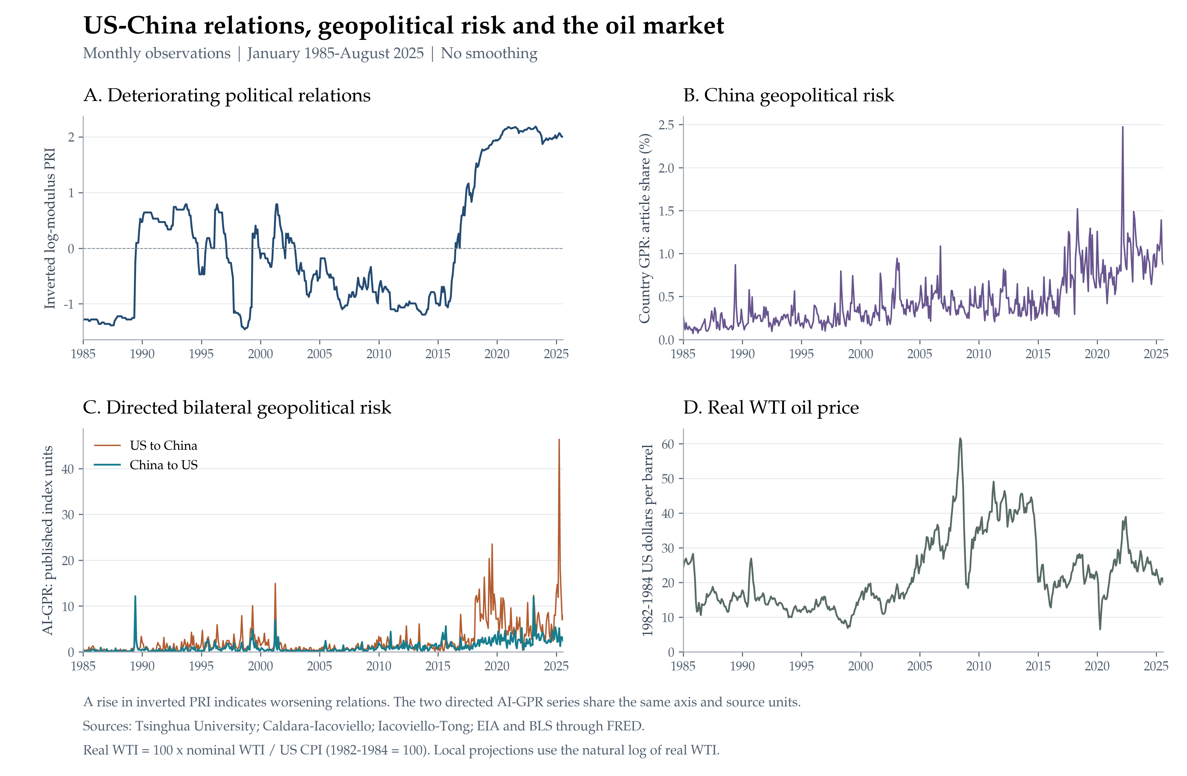
The following correlations use the same 488 monthly observations for every pair. PRI enters in its inverted log-modulus form, as defined above. Real WTI enters in levels here, as plotted; the local projections below use its natural logarithm.
| Series | Inverted PRI | China GPR | China → US | US → China | Real WTI |
|---|---|---|---|---|---|
| Inverted log-modulus PRI | 1.000 | 0.636 | 0.492 | 0.579 | −0.143 |
| China GPR | 0.636 | 1.000 | 0.548 | 0.583 | 0.243 |
| China → US | 0.492 | 0.548 | 1.000 | 0.586 | 0.076 |
| US → China | 0.579 | 0.583 | 0.586 | 1.000 | −0.013 |
| Real WTI | −0.143 | 0.243 | 0.076 | −0.013 | 1.000 |
The political indicators share information without being interchangeable: their contemporaneous correlations range from 0.492 to 0.636. Their relationships with real oil prices are weaker. Over the full sample, inverted PRI is negatively correlated with real WTI (−0.143), while China GPR has a positive correlation (0.243). The two directed indices have correlations close to zero with oil prices.
The distinction between persistent movements and monthly changes is revealing. The correlation between inverted PRI and China GPR falls from 0.636 in levels to 0.024 in first differences. The two directed indices retain a stronger association in monthly changes (0.389, compared with 0.586 in levels). The first-difference comparisons use 487 observations, from February 1985 to August 2025. This pattern suggests that part of the overlap between political relations and China GPR reflects persistent variation, while the directed indices also share shorter-term movements.
The oil-price relationship also depends on the sample: the inverted PRI–real WTI correlation is −0.407 over January 2000–August 2025 (308 observations), compared with −0.143 over the full period. These descriptive correlations motivate the sample comparisons below. They measure contemporaneous, unconditional co-movement; the local projections examine subsequent oil-price responses conditional on the model’s controls.
A direct local-projection specification
The local-projection framework follows Jordà (2005). Jordà and Taylor (2025) provide a comprehensive review of its specification, identification and inference.
Let \(y_t\) be the natural logarithm of the real WTI oil price, obtained by deflating nominal WTI with the US CPI. Define the oil-market controls as
where \(Q_t\) is world crude-oil production and \(A_t\) is world industrial production. For the inverted PRI, the regression at each horizon is
The China GPR comparison replaces \(R_t\) and its lags with the China GPR series. For the directed indices, both current directions enter together:
These are constant-coefficient local projections estimated in one step. They include an intercept and exactly 24 lags of each listed variable. The dependent variable is the future log price level; the plotted coefficients are not sums of successive responses. The current political indicator enters directly, without a preliminary shock-extraction regression. The causal interpretation rests on conditional short-run exogeneity, explained below.
This makes the exercise a one-step replication of the earlier qualitative finding, using an updated data vintage and an explicit common sample. Exact numerical reproduction of the published estimates is not claimed. The directed-index results are an extension of the original analysis.
Identification: conditional short-run exogeneity
The identifying assumption is short-run exogeneity conditional on the included controls. Conditional on 24 monthly lags of the political indicator(s) and oil-market variables—and, in the joint specification, the other contemporaneous directed index—the current index movement is treated as exogenous with respect to the oil-market disturbances represented in the horizon-specific errors. Under this assumption, the local-projection coefficients identify the dynamic oil-price response to a geopolitical innovation. The one-step regression isolates this conditional variation directly; it does not require a preliminary shock-extraction regression.
The economic rationale is that diplomatic and security developments can change political relations or geopolitical-risk news within a month for reasons that do not respond to contemporaneous idiosyncratic oil-price innovations. Lagged oil production, global activity and oil prices absorb the observed recent state of the oil market; conditioning on the other current directed index separates the two contemporaneous news signals. This is a maintained timing and information assumption: lag controls do not establish it by themselves. Contemporaneous omitted news affecting both the index and oil prices, or an immediate political response to oil-price developments, would threaten the causal interpretation.
Each response is scaled as
where \(s\) is one conditional standard deviation of the relevant current index, calibrated on February 2000–September 2021. Each indicator’s scale remains fixed across the four sample windows. The vertical units are log-percentage points, approximately percentage changes for small responses. A response of \(r\) corresponds exactly to \(100[\exp(r/100)-1]\) percent. These are not elasticities, and the different indicators do not represent identical-unit interventions.
Four windows, with comparable dates across horizons
The estimates use four windows. The short labels on the figures describe data or outcome coverage; the table identifies the current-index dates actually used in every regression.
| Figure label | Current-index dates, all horizons | Last outcome month | Observations per horizon |
|---|---|---|---|
| 2000–2019 | February 2000–January 2016 | December 2019 | 192 |
| 2000–2025 | February 2000–September 2021 | August 2025 | 260 |
| 1990–2025 | January 1990–September 2021 | August 2025 | 381 |
| 1985–2025 | January 1987–September 2021 | August 2025 | 417 |
A common index date means that the same months \(t\) are retained at every horizon, from impact to month 47. This is a deliberate choice to hold the composition of the sample fixed as the horizon changes. Since the last available oil-price outcome is August 2025, the latest usable current-index month is September 2021. Events in 2022–2025 contribute to later outcomes, but movements in the political indices during those years do not enter as current regressors.
Extending the outcome window to 2025 adds 68 current-index months, from February 2016 through September 2021, covering the 2016 election and the first Trump presidency. This period matters economically because the ambition to reduce US dependence on China raised the prospect of a lasting change in the organization of trade and production. The implications of that decoupling agenda are discussed below.
The full dataset starts in January 1985. Its first 24 months supply the lagged regressors, so the first usable index date is January 1987. The 1990-start estimates use 1988–1989 observations for their initial lags.
The historical PRI result reappears
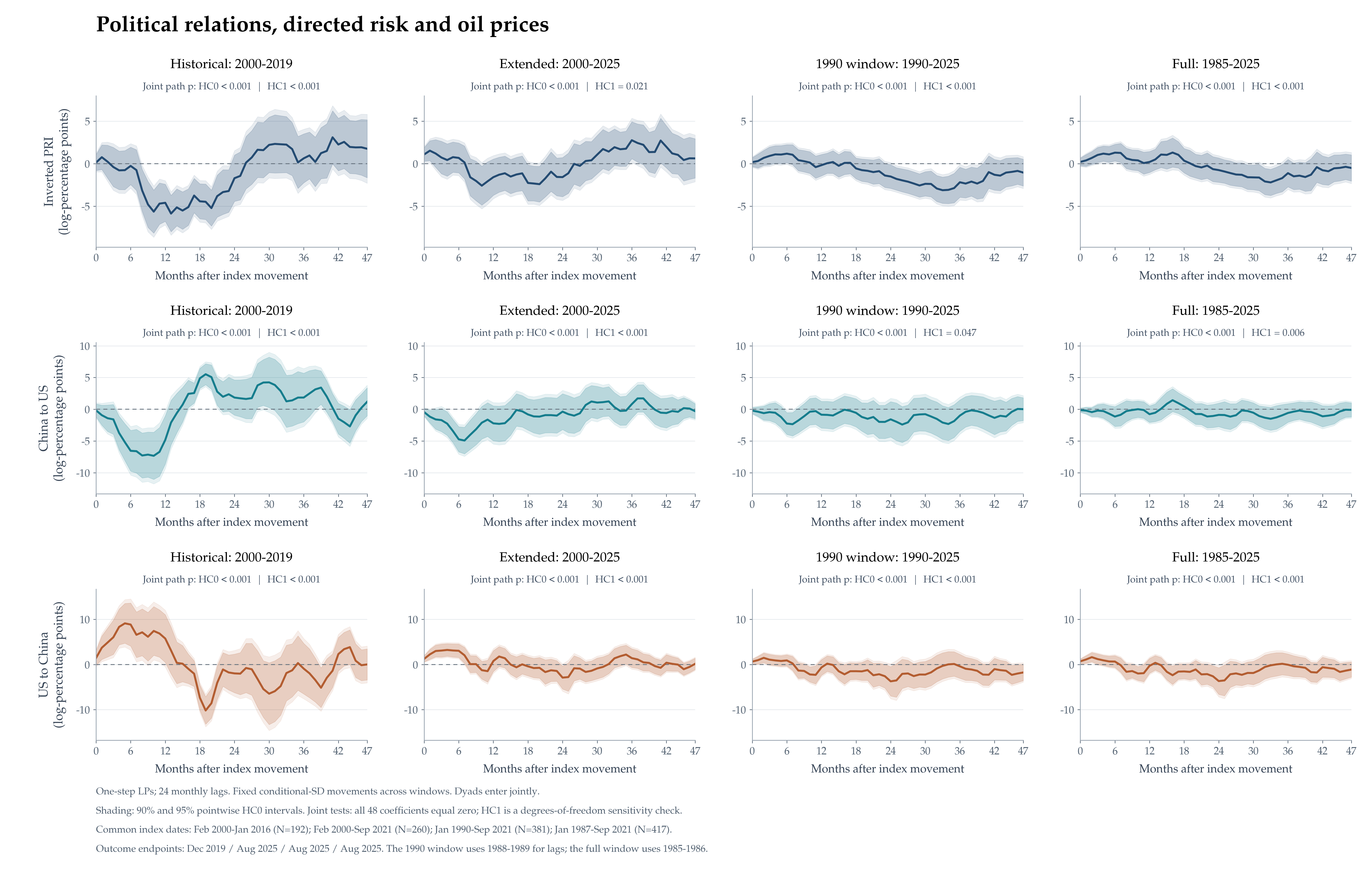
The first result is the clearest link with Mignon and Saadaoui. In the historical window, a deterioration in political relations is followed by a sustained negative oil-price response. At month 12, the estimate is −4.59 log-percentage points. The 95% pointwise interval excludes zero from months 8 to 23.
Click the figure to enlarge or reduce it. Scroll inside the enlarged image to read the notes.
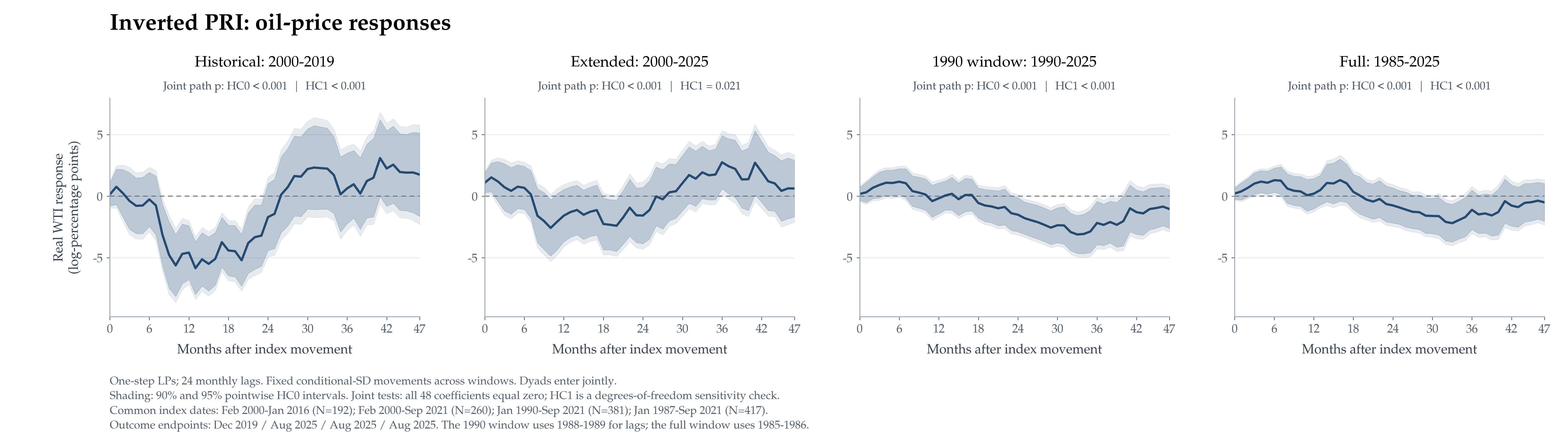
This pattern is consistent with weaker expected activity and oil demand following a deterioration in bilateral relations. The updated 2000-start window retains a jointly significant PRI path (HC1 p = 0.021), although its negative phase is less precisely located: it has some 90% pointwise rejections, but none at 95%. The joint rejection concerns the entire path, rather than that negative phase alone. Adding earlier observations changes the timing again, with the negative PRI response concentrated at substantially longer horizons.
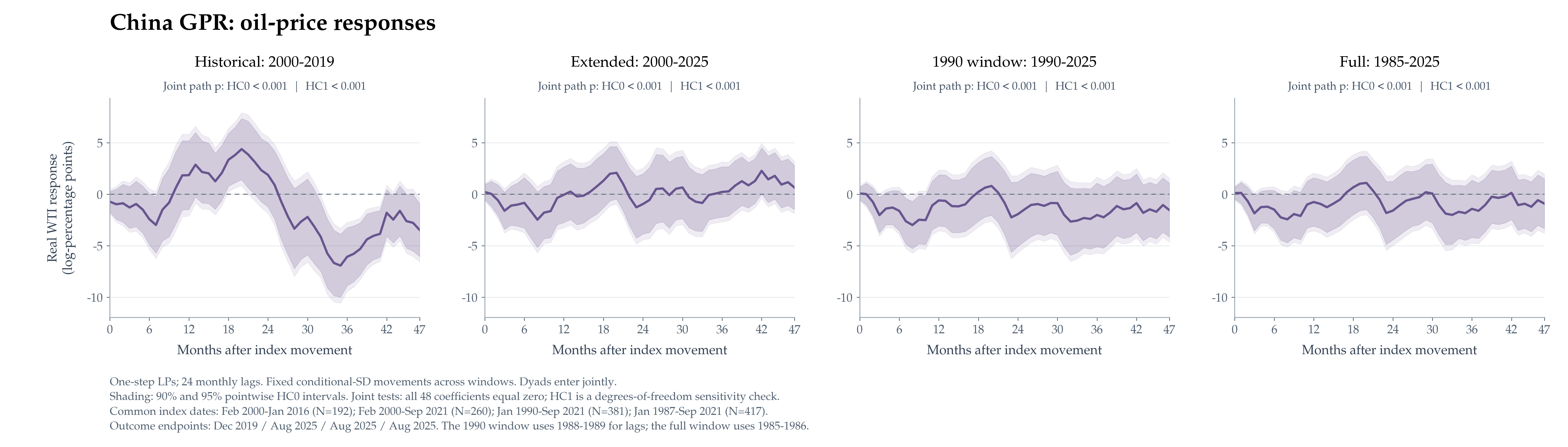
China GPR provides a useful contrast. In the historical window, its response turns positive around months 18–21 before becoming negative later. In the extended 2000-start window, no individual horizon excludes zero at 95%. Nevertheless, the extended China GPR path rejects the all-zero null (HC1 p = 0.000139). The joint test supports an overall response, even though a stable positive response across periods is not established.
Click the figure to enlarge or reduce it. Scroll inside the enlarged image to read the notes.
Does the direction of geopolitical news matter?
In the joint specification, an increase in China → US risk is followed by an early decline in oil prices in both 2000-start windows. At month six, the estimated response is −6.55 log-percentage points in the historical window and −4.74 in the extended window. Both exclude zero at 95% pointwise confidence.
Click the figure to enlarge or reduce it. Scroll inside the enlarged image to read the notes.
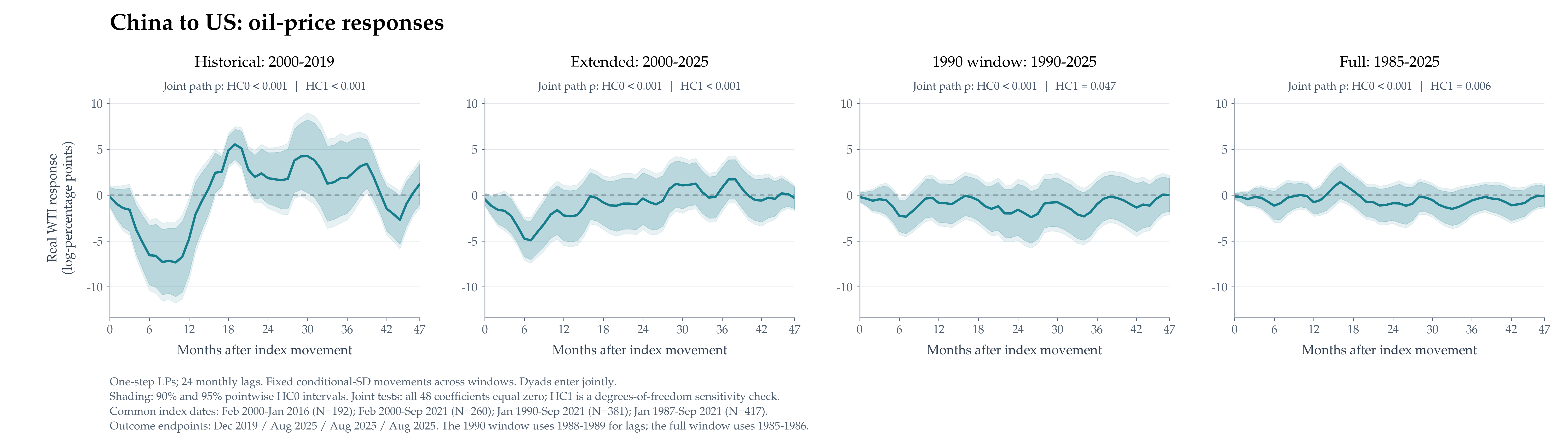
The early decline remains visible with a 1990 start: the month-six estimate is −2.25. With the full dataset beginning in 1985, it falls to −1.15 and is imprecisely estimated. No individual horizon of this earliest-start joint China → US response excludes zero at 90%, yet its full path is jointly significant (HC1 p = 0.0057). The 1990-start path also rejects zero, although its p-value of 0.0472 is close to the 5% threshold. The joint test provides the primary assessment of the overall response; pointwise intervals provide complementary information about particular horizons. The imprecise early coefficient therefore does not establish the absence of a response over the full horizon.
The US → China response initially goes in the opposite direction in the 2000-start windows. At month six, it is +8.84 in the historical window and +3.03 in the extended window. The full US → China path is jointly significant in all four windows (HC1 p < 0.001). The longer samples have smaller early estimates and a subsequent negative phase. At month 24, the joint estimate is −3.73 with a 1990 start and −3.67 using the full dataset; their pointwise p-values are 0.059 and 0.040, respectively.
Click the figure to enlarge or reduce it. Scroll inside the enlarged image to read the notes.
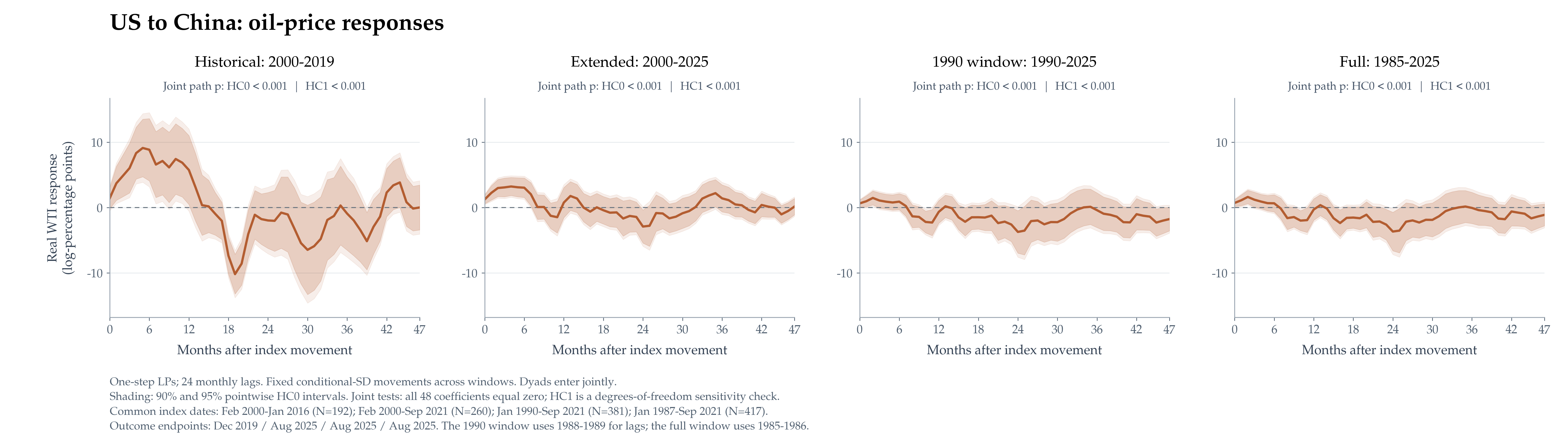
These estimates suggest that the two directions convey different conditional information. They do not establish that escalation by one country always raises oil prices while escalation by the other always lowers them.
Why contemporaneous conditioning matters
Equation (3) asks what happens after a movement in one directed index holding the other current index fixed. That qualification matters when the two series record overlapping geopolitical episodes.
A diagnostic regression removes the other current directed index while retaining all 24 lags of both directions and all oil-market controls. It uses the same observations and the same response scale. Thus the comparison isolates the change in contemporaneous conditioning.
Click the figure to enlarge or reduce it. Scroll inside the enlarged image to read the notes.
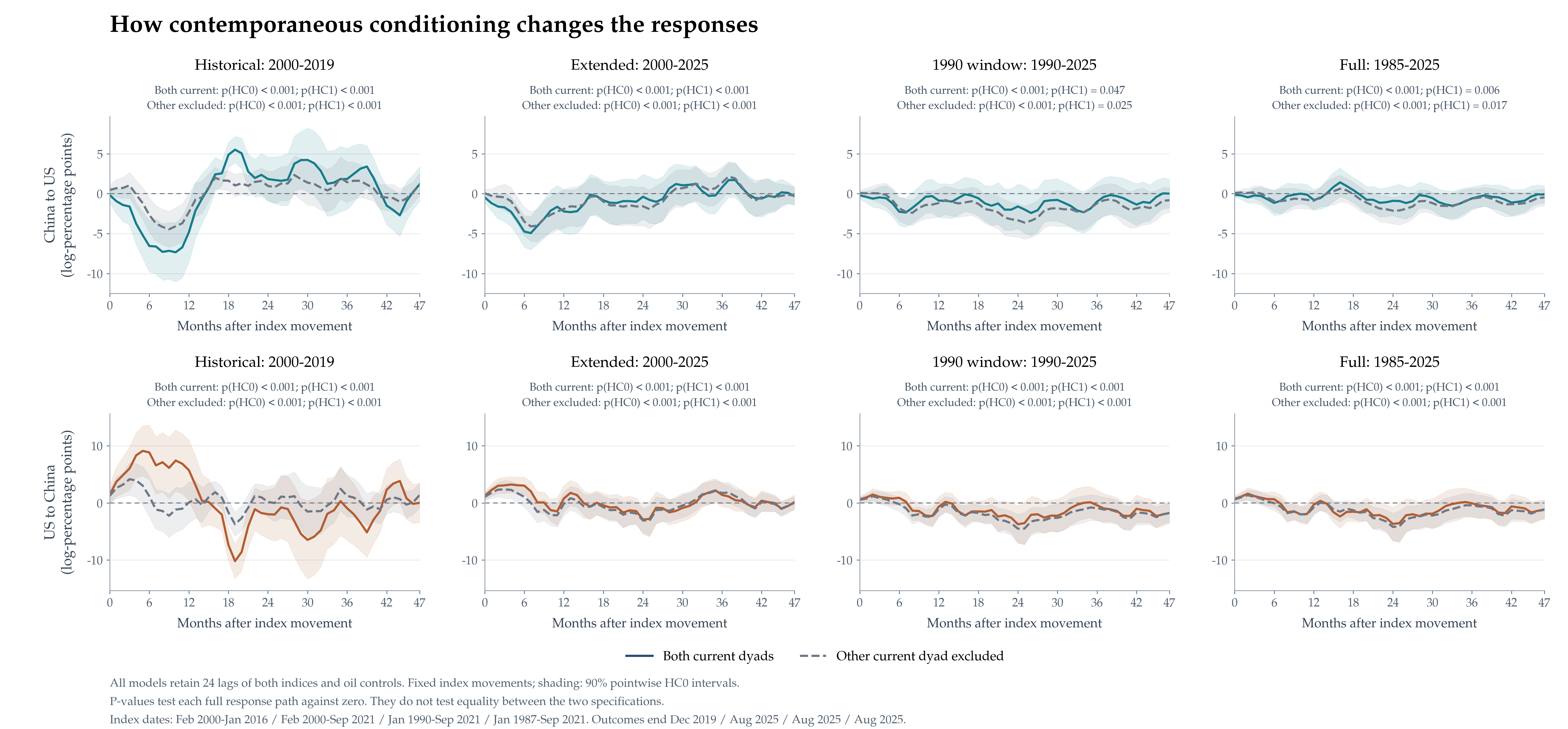
For the extended 2000-start window, the six-month comparison is particularly informative:
| Current index | Both current directions included | Other current direction excluded |
|---|---|---|
| China → US | −4.74 (p < 0.001) | −3.49 (p = 0.001) |
| US → China | +3.03 (p < 0.001) | +1.08 (p = 0.319) |
Entries are log-percentage-point responses; parentheses give HC0 pointwise p-values.
The China → US decline remains evident. The US → China estimate becomes much smaller and its interval includes zero. This change concerns the six-month coefficient: both entire paths remain jointly significant after excluding the other current index, with extended-sample HC1 p-values of 0.0000179 for China → US and 4.09 × 10⁻¹⁷ for US → China. Part of the striking opposite-sign pattern therefore depends on separating contemporaneously correlated signals. It should not automatically be read as evidence of two opposite structural mechanisms.
What do the longer samples add?
The 1990–2025 estimates provide a bridge between the post-2000 comparison and the fullest available dataset. They retain an early negative China → US response, but move the negative PRI phase to roughly two to three years after the index movement. The PRI’s 95% pointwise interval is below zero at months 25–39.
Click the figure to enlarge or reduce it. Scroll inside the enlarged image to read the notes.
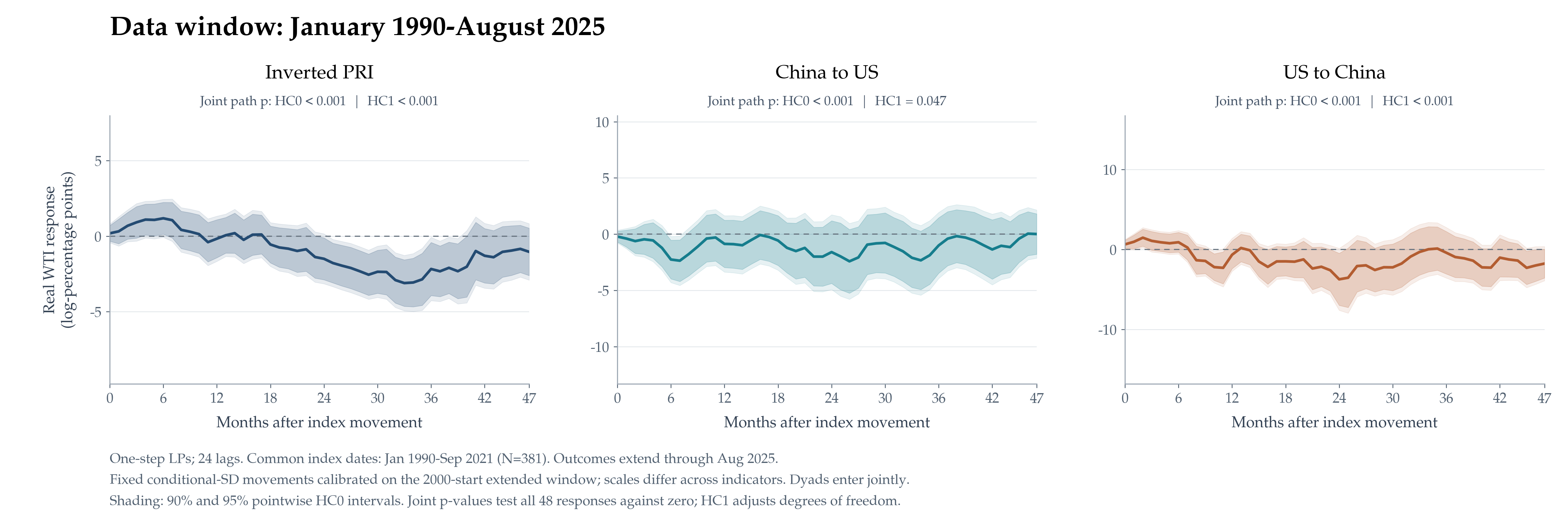
Using all data from 1985 further weakens the early China → US decline. For PRI, the month-six estimate is now positive, while the response around month 33 is −2.19 log-percentage points. Its 95% pointwise interval is negative at months 32–34. The US → China profile still contains a later decline.
Click the figure to enlarge or reduce it. Scroll inside the enlarged image to read the notes.
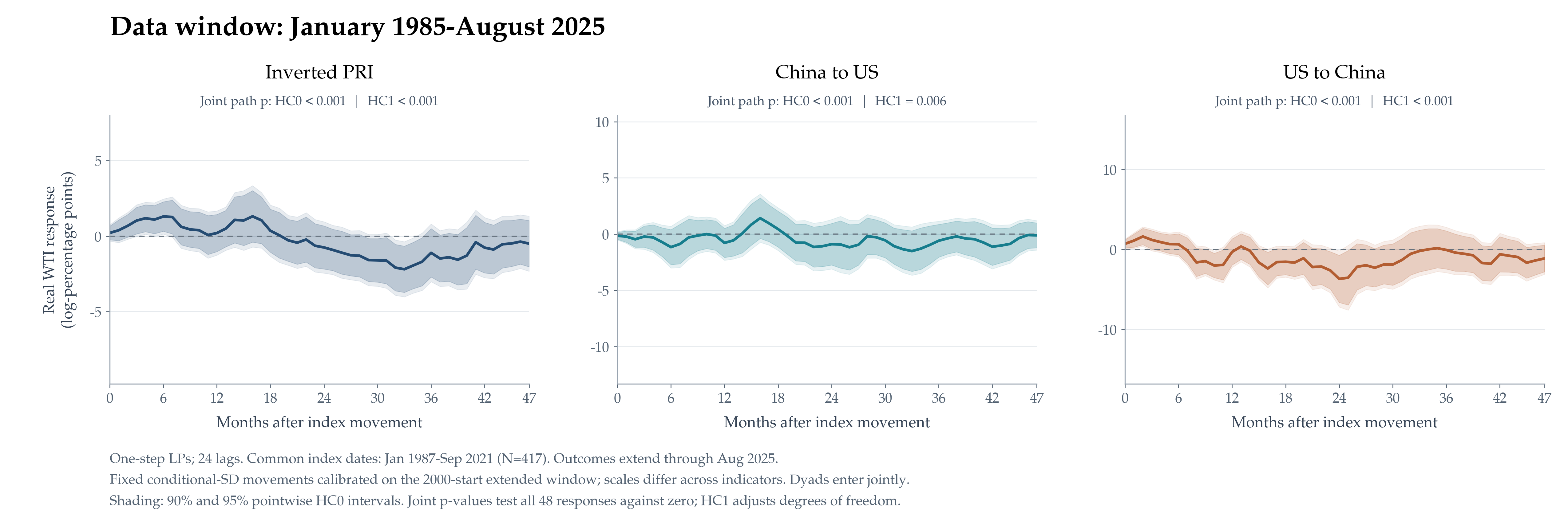
These are nested pooled samples, not separate regime estimates. Their differences reveal sensitivity to the observations included, but do not constitute a formal test of a structural break. All four windows also use the same updated data vintage.
The combined figure gathers the three main indicators in one view. It highlights both the historical negative PRI phase and the substantial changes in timing and magnitude when the observation window expands.
Click the figure to enlarge or reduce it. Scroll inside the enlarged image to read the notes.
Why joint-path testing takes priority
For the question of whether oil prices respond over the full horizon, joint testing takes priority over individual-horizon testing. As emphasized by Jordà and Taylor (2025), the two forms of inference answer different questions. A pointwise interval assesses one month. The joint test evaluates whether all 48 population responses \(r_h=100s\beta_h\) for an indicator are zero together:
Let \(\widehat{\mathbf r}=(\widehat r_0,\ldots,\widehat r_{47})'\) and let \(\widehat V\) estimate its covariance matrix. The Wald statistic and reported asymptotic p-value are
The covariance accounts for correlation between the estimated responses at different horizons. The figures report HC0 and HC1 versions. HC1 multiplies the HC0 covariance by \(N/(N-K)\), where \(K\) includes the intercept and all estimated regression coefficients. The HC1 p-values are:
| Indicator | 2000–2019 | 2000–2025 | 1990–2025 | 1985–2025 |
|---|---|---|---|---|
| Inverted PRI | < 0.001 | 0.021 | < 0.001 | < 0.001 |
| China → US, joint | < 0.001 | < 0.001 | 0.047 | 0.006 |
| US → China, joint | < 0.001 | < 0.001 | < 0.001 | < 0.001 |
| China GPR | < 0.001 | < 0.001 | < 0.001 | < 0.001 |
Every one of the 16 primary indicator–sample combinations rejects an entirely zero response at the nominal 5% level under the retained HC1 convention. For PRI, the rejection survives the extension through 2025 (p = 0.021). For China → US, the 1990-start result is the weakest joint rejection (p = 0.0472), while the full 1985-start path rejects at p = 0.0057. The US → China and China GPR paths reject in all four windows with p-values below 0.001.
The full-sample China → US and extended China GPR figures are particularly revealing: their individual intervals provide little evidence at specific horizons, yet the corresponding joint tests reject an all-zero path. Similarly, removing the other current directed index weakens the early positive US → China coefficient without eliminating the joint significance of its entire path.
The overall inference should therefore be led by the joint path test, rather than by counting individually significant months. Failure to reject zero at individual horizons does not imply that the full path is insignificant. The Wald test uses the covariance across horizons, so combinations of coefficients can be estimated precisely even when individual coefficients are not. Pointwise intervals remain useful for assessing uncertainty at particular months.
Joint rejection provides evidence against an entirely zero path within the maintained inferential framework; it does not establish significance at every horizon, a constant sign, or differences between directions or samples. The 16 results are separate nominal tests, without adjustment across that collection, and statistical significance alone does not identify the economic mechanism.
The inference deserves care. The retained covariance uses same-date score cross-products across horizons; it does not add cross-date HAC terms. Its validity therefore requires appropriate assumptions on the temporal dependence of the regression scores. The specification’s 24 lags alone do not establish those assumptions. HC1 is a degrees-of-freedom adjustment, not a complete finite-sample correction. This matters especially in the historical joint model, with 192 observations, 123 coefficients per horizon and 48 restrictions in the path test. The very small p-values should be interpreted within that inferential setup.
Economic interpretation: decoupling, demand and supply risk
The historical PRI result is consistent with a demand-expectations channel. A durable deterioration in US–China relations may lower expected trade, investment and manufacturing activity. Through production networks, the consequences can extend beyond the two countries. Expected oil demand then weakens, and the oil price can fall even though geopolitical tensions have risen.
Trump’s decoupling agenda gives this demand channel a concrete economic interpretation. His administration introduced tariffs on Chinese industrial goods in 2018; in September 2020, Trump explicitly presented decoupling and tariffs as ways to end US reliance on China and bring manufacturing home. Such announcements could change expectations about the durability of economic integration. Firms facing uncertain market access and lasting restrictions may postpone investment, reduce orders and reorganize production networks. If weaker global activity outweighs the relocation of production elsewhere, expected oil demand can fall. Political deterioration would then signal a persistent change in trade and production, rather than a temporary diplomatic disagreement. This mechanism could contribute to negative responses over subsequent years, even if an initial increase reflects supply concerns or precautionary demand. The pooled estimates do not separately identify the effect of decoupling policies.
The early China → US decline in the 2000-start samples fits that account. One possible explanation is that some forms of escalation provide a particularly strong signal of restrictions that will be implemented and sustained. This is a “walk the talk” hypothesis about the information in political news. The regressions do not directly measure diplomatic credibility or subsequent implementation, so the hypothesis remains to be tested.
A positive oil-price response requires a price-increasing channel as well. Anticipated supply disruption or precautionary inventory demand could temporarily outweigh weaker expected activity. Simply describing diplomacy as unpredictable would not explain why the price rises. Moreover, the early US → China response shrinks markedly when the other current directed index is excluded, which cautions against attributing it entirely to a distinct supply-risk mechanism.
The next empirical step would connect the indices to subsequent trade, industrial production, inventories and policy implementation, while distinguishing threats from realized actions. For now, the evidence supports a more specific conclusion: political deterioration can be followed by lower oil prices, and the direction of reported tensions helps describe that relationship, but the estimated timing and strength depend on sample coverage and contemporaneous conditioning.
Technical note on scaling and covariance
For each index, \(s\) is the standard deviation of its residual after projection on the other regressors in the calibration sample. For the joint dyad model, those regressors include the other current directed index. The figures therefore show the oil-price response to an increase of one conditional standard deviation, measured in each index’s own units: 0.086234 for transformed, inverted PRI; 0.517331 for China → US; 1.373233 for US → China; and 0.137545 for China GPR. These numbers specify the size of the index increase, not the size of the oil-price response. Each increase is kept identical across the four estimation windows, so sample comparisons reflect changes in estimated responses rather than changes in normalization. The conditioning diagnostic also retains the joint-model scale for each direction.
To make the path test explicit, let \(z_t\) be the residual from projecting the current index on the other regressors in the estimation window. Let \(\widehat\varepsilon_{t+h,h}\) be the horizon-specific residual. With \(a=100s\), define
Then the two covariance estimates are
Here \(K=98\) for PRI and China GPR, 123 for the joint dyad model, and 122 for the conditioning diagnostics. The shaded bands in the figures remain pointwise HC0 normal intervals; they are not simultaneous confidence bands for the full path.
A related paper examining political relations, geopolitical risk and oil prices has been submitted to a journal.
Data and references
The dataset contains 488 monthly observations from January 1985 to August 2025. The PRI uses the Tsinghua release dated 4 December 2025. Real WTI is \(100\times\mathrm{WTISPLC}/\mathrm{CPIAUCSL}\); world oil production is crude oil including lease condensate; world industrial production covers the OECD plus six major emerging economies. All comparisons retain the data vintage stored with this exercise.
- Mignon, V., and J. Saadaoui (2024). “How do political tensions and geopolitical risks impact oil prices?” Energy Economics, 129, 107219. Article · Earlier EconMacro presentation.
- Jordà, Ò. (2005). “Estimation and Inference of Impulse Responses by Local Projections.” American Economic Review, 95(1), 161–182. Article.
- Jordà, Ò., and A. M. Taylor (2025). “Local Projections.” Journal of Economic Literature, 63(1), 59–110. Article.
- Caldara, D., and M. Iacoviello (2022). “Measuring Geopolitical Risk.” American Economic Review, 112(4), 1194–1225. Article · GPR data.
- Iacoviello, M., and J. Tong (2026). “The AI-GPR Index: Measuring Geopolitical Risk using Artificial Intelligence.” Working paper, 25 September. Paper · Data and documentation.
- Montiel Olea, J. L., and M. Plagborg-Møller (2021). “Local Projection Inference Is Simpler and More Robust Than You Think.” Econometrica, 89(4), 1789–1823. Paper.
- PRI source: Tsinghua University, Institute of International Relations, China’s relations with major countries.
- Oil-market data: EIA and BLS through FRED, WTI and CPI; EIA world crude-oil production; world industrial production from Christiane Baumeister’s data page.