Should an inflation-targeting central bank respond directly to the real exchange rate? A small theoretical model can make this question surprisingly concrete. The central bank chooses a rule for its real interest rate; that rule changes the way shocks affect output, inflation, and the exchange rate; and these responses determine the losses associated with different policy choices.
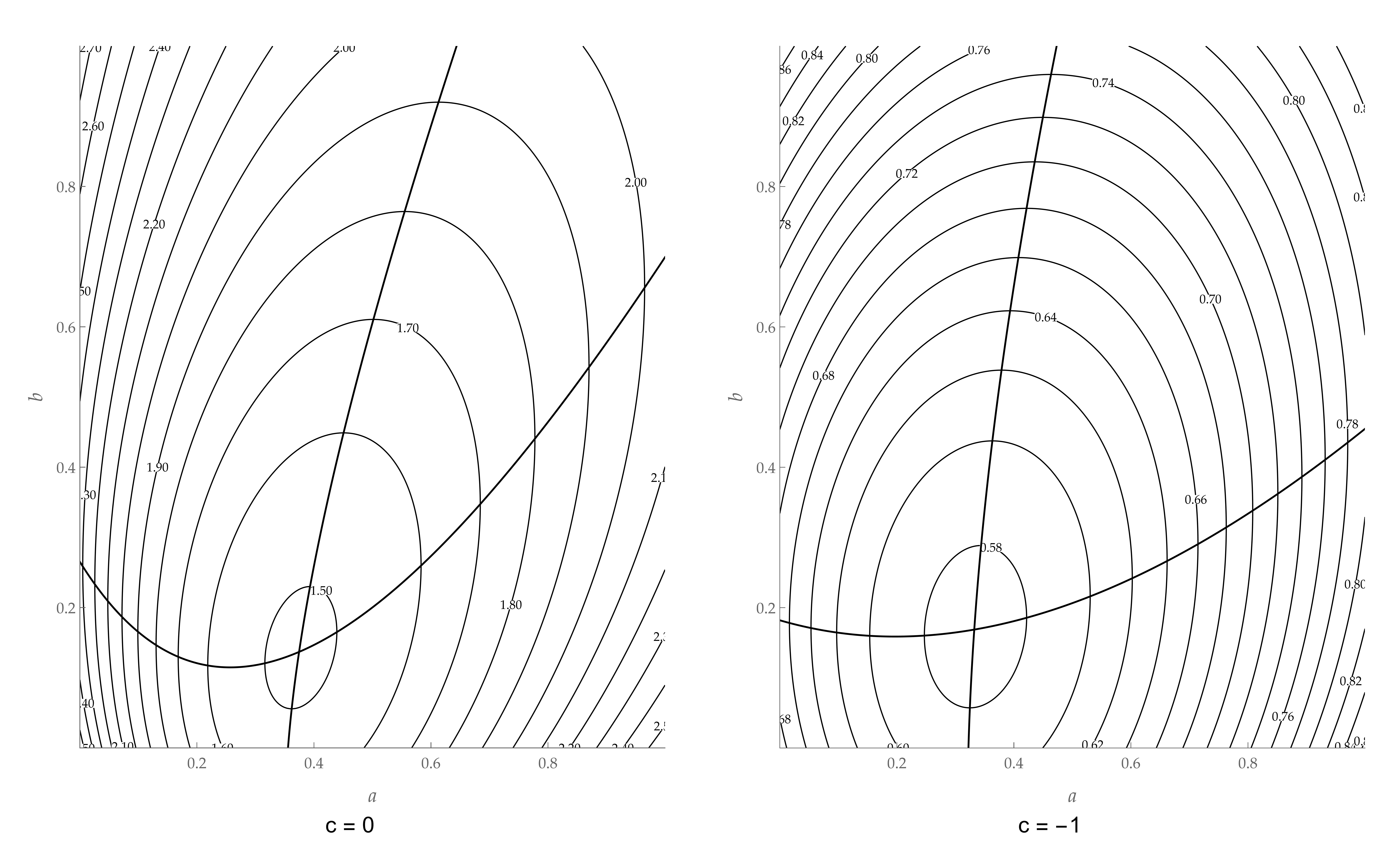
In Appendix A of Aizenman, Hutchison, and Noy (2011), Inflation Targeting and Real Exchange Rates in Emerging Markets, Figure A.1 summarizes this mechanism with two contour plots. My starting point was a practical replication exercise, using a Mathematica notebook prepared by my friend Mario. Reconstructing the figure led to a useful distinction: a formula can closely reproduce a published graph while differing from the formula implied by the model’s equations.
This question belongs to a wider literature on monetary-policy rules. Taylor (1993) provides a reference point for systematic interest-rate responses to inflation and output. Ball (1999) studies how exchange-rate transmission changes the design of rules in open economies. Svensson (2000) examines strict and flexible inflation targeting in a forward-looking open-economy model. These studies provide economic context; the calculations below solve the four equations stated in the Aizenman–Hutchison–Noy appendix.
The post has two parts. Part I develops the economic model and the algebra: we solve the equations by substitution, calculate the variances, construct the policy loss, and interpret the figures. Part II opens the Mathematica notebook: we follow the actual instructions that implement those calculations, check the solution, and explore sensitivity. As in my previous post on the FEER-SMIM model, the aim is to make the connection between economic equations and computational implementation transparent.
The scope is specific. This is a reconstruction of the theoretical illustration in Appendix A, pages 722–723. It does not re-estimate the paper’s empirical results. The two implementations below are labeled throughout: \(L_S\) follows the stated structural equations, whereas \(L_R\) is an inferred objective that closely reproduces the published figure. The original authors’ simulation code has not been obtained.
Part I. The model and its results
1. The economic question and the loss function
Consider a central bank that dislikes fluctuations in inflation and output. A familiar quadratic objective is a weighted sum of their variances. Appendix A adds a third concern: exchange-rate volatility may reduce potential output, for example through economic mechanisms that make unstable relative prices costly. The appendix represents that concern by adding an exchange-rate variance term:
Here \(V(x)\) means the variance of \(x\). Inflation has a normalized weight of one; \(\mu\) measures the relative importance of output stability; and \(\phi\) measures the cost attached to exchange-rate variability. These weights are preferences in a theoretical calculation. They are not estimated regression coefficients in this exercise.
The variables are deviations from their average or reference levels. With zero-mean shocks and a well-defined linear solution, the endogenous deviations also have zero means. Consequently, \(V(y)=E[y^2]\), and similarly for inflation and the exchange rate. A large positive deviation and a large negative deviation both contribute to the quadratic loss.
What the central bank chooses is a policy rule. It selects coefficients describing how its real interest rate reacts to inflation, output, and the exchange rate. For each candidate rule, the model delivers a different response to each shock and therefore a different value of \(L\).
The distinction between stabilizing inflation alone and balancing several objectives is central to flexible inflation targeting. Svensson (2000) analyzes that distinction in a model with expectations and transmission lags. Here, the positive output weight makes the same broad trade-off visible in a static calculation, while the exchange-rate variance term is an explicit feature of this appendix’s specified objective.
The exercise proceeds in this order:
- Choose candidate policy coefficients.
- Solve the simultaneous equations under that policy.
- Calculate the variances generated by the shocks.
- Combine those variances into a loss.
- Compare losses across policies.
No historical time series is needed for this theoretical calculation. Once the structural parameters, shock variances, and policy coefficients are specified, the variances can be calculated analytically.
2. The four equations, one at a time
The appendix uses a static version of an open-economy model: adjustment occurs within the period, without persistence. We therefore solve all four equations together. We are not tracing a dynamic impulse response over several periods.
| Symbol | Meaning in this appendix |
|---|---|
| \(y\) | Output deviation from its reference level. |
| \(\pi\) | Inflation deviation. |
| \(e\) | Real exchange-rate deviation; a higher value means an appreciation. |
| \(r\) | Real interest-rate deviation. |
| \(\varepsilon,\eta,\nu\) | Demand, inflation, and exchange-rate shocks. |
| \(\alpha,\beta,\gamma,\delta,\theta\) | Positive structural parameters describing economic transmission. |
| \(a,b,c\) | Policy-rule coefficients chosen for the illustration. |
2.1 Output: the open-economy IS equation
A higher real interest rate reduces demand through \(-\beta r\). An appreciation reduces output through \(-\delta e\), consistent with a deterioration in price competitiveness. A positive demand shock \(\varepsilon\) increases output. The coefficients describe partial effects within this equation; the final equilibrium response also includes feedback through the other equations.
2.2 Inflation: the open-economy Phillips equation
Higher output raises inflation. An appreciation lowers inflation directly, through the exchange-rate term, which represents a channel such as cheaper imports. The shock \(\eta\) captures inflationary disturbances that are not explained by output or the exchange rate.
2.3 The exchange rate
A higher real interest rate appreciates the currency in this stylized relationship. The shock \(\nu\) collects other exchange-rate influences. The positive sign before \(\theta r\) is consistent with the appendix’s convention: higher \(e\) means appreciation.
2.4 The policy rule
The central bank’s real interest rate responds to the three endogenous variables. Figure A.1 compares \(c=0\) with \(c=-1\), while allowing \(a\) and \(b\) to vary between zero and one.
When \(c=0\), the rule has no direct exchange-rate term. Exchange rates still matter indirectly because they affect output and inflation. When \(c\lt0\), a depreciation, meaning \(e\lt0\), makes \(ce\) positive. Holding the other rule terms fixed, that depreciation calls for a higher real interest rate. This is the sign convention behind the comparison.
Ball (1999) explains why an open-economy rule must account for monetary transmission through both interest rates and exchange rates. That is the motivation for inspecting the exchange-rate term here. His dynamic model and the present static illustration are different, so a numerical coefficient from one should not be imported into the other without re-solving the model. Likewise, the variable \(r\) here is a real-rate deviation, whereas Taylor’s original illustrative rule is expressed for the nominal federal funds rate.
2.5 Why these equations must be solved together
The rule determines \(r\) using \(\pi\), \(y\), and \(e\), but those variables themselves depend on \(r\). Substituting a value into only one equation cannot complete the calculation. The model requires a mutually consistent set of four values.
Readers of the previous matrix-form post can recognize the same problem immediately:
Each row is one of the four original equations rearranged to put endogenous variables on the left. This is a \(4\times4\) system. The substitution steps below solve precisely this system and reveal the economic content of its denominator.
3. Solving for the policy rate step by step
The four equations must hold simultaneously. Substitution lets us solve them by first expressing output, inflation, and the exchange rate in terms of the interest rate and the shocks, and then using the policy rule to determine the interest rate itself. Throughout this calculation, the structural parameters and policy coefficients are fixed. Recall that \(\varepsilon\) is the demand shock, \(\eta\) is the inflation shock, and \(\nu\) is the exchange-rate shock.
The endogenous variables retain their earlier meanings: \(y\) is output relative to its reference level, \(\pi\) is inflation relative to its reference level, \(e\) is the real exchange-rate deviation, and \(r\) is the real interest-rate deviation. A positive \(e\) denotes appreciation. The letters \(a,b,c\) are policy-rule coefficients. They are distinct from the structural parameters \(\alpha,\beta,\gamma,\delta,\theta\); for example, changing \(a\) changes the policy response to inflation, whereas changing \(\alpha\) changes how output enters the inflation equation.
3.1 Substitute the exchange-rate equation into output
Start from \(y=-\beta r-\delta e+\varepsilon\) and replace \(e\) with \(\theta r+\nu\). Distribute the minus sign across both terms:
Define \(B\equiv\beta+\delta\theta\). The coefficient combines the direct interest-rate effect on output, \(\beta\), and the effect through interest-rate-induced appreciation, \(\delta\theta\). We obtain
The term \(-Br\) already includes both interest-rate channels. To see this, hold the shocks fixed and consider an increase in \(r\): output changes directly through \(-\beta r\), while the induced appreciation \(\theta r\) changes output through \(-\delta\theta r\). The separate term \(-\delta\nu\) captures the part of appreciation originating from the exchange-rate shock itself. Calling this last contribution direct means holding the interest rate fixed; it still operates through the exchange rate in the original output equation.
3.2 Express inflation in terms of the interest rate
Now use \(\pi=\alpha y-\gamma e+\eta\). Substitute the expressions for both \(y\) and \(e\), expand, and collect the interest-rate terms:
The coefficient \(\alpha B+\gamma\theta\) combines two channels through which a higher interest rate lowers inflation: reduced output and appreciation. This expression still contains the endogenous interest rate; the next step determines it.
Writing the equation this way does not assume that the interest rate changes before output or inflation. The model is simultaneous: all four variables are determined together for a given realization of the shocks. The order of substitution is an algebraic method for finding that common solution, rather than a timeline of economic adjustment.
3.3 Substitute into the policy rule and collect terms
The policy rule is \(r=a\pi+by+ce\). Replace each variable on its right-hand side:
Expanding the three brackets gives
Group terms according to whether they multiply the interest rate, the demand shock, the inflation shock, or the exchange-rate shock:
Why does the coefficient on the left start with one? The original left-hand side is \(r=1\times r\). Add \((a\alpha B+a\gamma\theta+bB-c\theta)r\) to both sides of the last equation. This cancels its negative counterpart on the right. The left-hand side becomes
Factoring out \(r\) preserves its original coefficient of one. The operation is the same as \(r+2r=(1+2)r\). Thus, after collecting the interest-rate terms, the equation is
Introduce the abbreviations
For \(H\), the terms \(a\alpha B+bB\) combine into \(Bq\), while \(a\gamma\theta-c\theta=\theta(a\gamma-c)\). For later use, expand and regroup \(k\):
Where does the demand-shock term \(q\varepsilon=(b+a\alpha)\varepsilon\) come from? A demand shock is an exogenous change in spending represented by \(\varepsilon\) in \(y=-\beta r-\delta e+\varepsilon\). Holding the interest rate and exchange rate fixed, a positive shock raises output. In the simultaneous solution, those two variables also respond.
Trace the terms multiplying \(\varepsilon\) in the two relevant components of the policy rule:
The demand shock enters the substituted output equation with coefficient one; multiplying output by \(b\) gives \(b\varepsilon\). It enters the substituted inflation equation with coefficient \(\alpha\); multiplying inflation by \(a\) gives \(a\alpha\varepsilon\). Add these two contributions and factor out their common shock:
The remaining policy component is \(ce=c\theta r+c\nu\). It contains no separate \(\varepsilon\) term at this stage; its feedback through \(r\) has already entered \(H\). Thus, \(q\) is the demand-shock coefficient in \(Hr\). The actual interest-rate loading is \(q/H\), obtained below.
The other two numerator coefficients can be traced in the same way. The inflation shock contributes \(a\eta\) through \(a\pi\). For the exchange-rate shock, collect the contributions from all three policy components:
These are contributions before the common feedback adjustment. The signs of the complete equilibrium responses must be read from \(q/H\), \(a/H\), and \(k/H\).
3.4 Divide by the common denominator
The collected equation is \(Hr=q\varepsilon+a\eta+k\nu\). Provided \(H\ne0\), divide by \(H\):
This is the interest-rate solution: its right-hand side contains only shocks and fixed coefficients. Separate its three terms to read the responses:
| Shock studied | Other shocks set to zero | Interest-rate response | Loading |
|---|---|---|---|
| Demand, \(\varepsilon\) | \(\eta=\nu=0\) | \(r=(q/H)\varepsilon\) | \(q/H\) |
| Inflation, \(\eta\) | \(\varepsilon=\nu=0\) | \(r=(a/H)\eta\) | \(a/H\) |
| Exchange rate, \(\nu\) | \(\varepsilon=\eta=0\) | \(r=(k/H)\nu\) | \(k/H\) |
For example, choosing \(a=0.4\), \(b=0.2\), and \(c=0\), with \(\alpha=0.4\), \(B=1\), \(\gamma=0.2\), and \(\theta=2\), gives \(q=0.2+0.4(0.4)=0.36\) and \(H=1+1(0.36)+2[0.4(0.2)-0]=1.52\). A unit demand shock therefore changes the interest rate by \(0.36/1.52\approx0.236842\). The numerator \(0.36\) becomes an equilibrium loading only after this division.
\(H\) is a combination of parameters and policy coefficients, not another shock. It summarizes the simultaneous feedback in the model and remains fixed when we vary a shock while holding those coefficients fixed. If \(H=0\), this division is invalid and the system does not have the unique solution used here.
The leading one in \(H\) is especially easy to miss. It comes from the original interest rate on the left of the policy rule: \(r=1\times r\). Moving the additional interest-rate terms from the right-hand side adds their coefficients to this one. Later, when the policy coefficients are optimized, changing \(a,b,c\) generally changes \(H\) as well as the shock numerators.
4. Recovering output, inflation, and the exchange rate
We now substitute the interest-rate solution back into the remaining equations. The resulting coefficients are shock loadings. A loading identifies which variable responds to which shock: the coefficient multiplying \(\eta\) in the output equation is an inflation-shock loading on output. The responding variable and the source of the shock are different pieces of information.
To isolate one loading, set the other two shocks to zero and leave the selected shock free to vary. This operation does not set output, inflation, or the exchange rate to zero in advance. Their responses are what the model determines. A one-unit shock is a convenient way to read the resulting coefficient; linearity then scales the response for any other shock size.
4.1 Recover output and simplify its three coefficients
Start from \(y=\varepsilon-Br-\delta\nu\) and substitute \(r=(q\varepsilon+a\eta+k\nu)/H\):
Multiply every term by \(H\), expand, and collect the shocks:
Here \(Hy\) means \(H\times y\); multiplying by \(H\) has simply cleared the denominator. We now examine output’s response to each shock. In every case, first identify where the coefficient comes from, then simplify its numerator, and finally divide by \(H\).
Demand shock \(\varepsilon\). Set \(\eta=\nu=0\). Demand contributes \(+\varepsilon\) directly to the substituted output equation, while the interest-rate response contributes \(-B(q/H)\varepsilon\):
Thus, \(H-Bq\) is the coefficient in \(Hy\), and \((H-Bq)/H\) is the coefficient in \(y\). Substitute the definition of \(H\):
Output’s demand-shock loading is consequently \([1+\theta(a\gamma-c)]/H\). The term \(1\) reflects the original demand impulse, and the full fraction includes the monetary-policy feedback. Its sign depends on the chosen coefficients.
Inflation shock \(\eta\). Set \(\varepsilon=\nu=0\). This shock has no separate additive term in the output equation; its effect enters through the interest rate:
The coefficient \(-aB\) is therefore the inflation-shock coefficient in scaled output \(Hy\). Output’s actual loading is \(-aB/H\). With positive \(a,B,H\), a positive inflation shock raises the policy rate and contracts output.
Exchange-rate shock \(\nu\). Set \(\varepsilon=\eta=0\). The interest rate is \(r=(k/H)\nu\). Substitute it into output:
The direct term \(-\delta\nu\) becomes \(-\delta H\nu/H\), which explains why its numerator contains \(H\). Now substitute \(k=c-a\gamma-\delta q\) and \(H=1+Bq+\theta(a\gamma-c)\):
The third line cancels \(B\delta q-\delta Bq\). The last line uses \(B-\delta\theta=\beta\), because \(B=\beta+\delta\theta\). The loading in \(y\) is \([\beta(a\gamma-c)-\delta]/H\). The negative direct output effect of appreciation can be partly offset, or reinforced, by the interest-rate response. Combining the three shocks gives
4.2 Recover the exchange rate and explain the numerator containing H
Recall \(e=\theta r+\nu\). Both the demand and inflation shocks affect the exchange rate through their effects on the interest rate. The exchange-rate shock also has its own additive term \(+\nu\). Substitute the full interest-rate solution:
Demand shock \(\varepsilon\). With \(\eta=\nu=0\), the interest rate is \(r=(q/H)\varepsilon\). Consequently,
Thus, \(\theta q\) is the coefficient in \(He\); the exchange rate’s actual demand-shock loading is \(\theta q/H\). A demand shock that raises the interest rate induces appreciation when \(\theta>0\).
Inflation shock \(\eta\). With \(\varepsilon=\nu=0\), substitute \(r=(a/H)\eta\):
The actual loading is \(a\theta/H\). With positive \(a,\theta,H\), the tightening following a positive inflation shock produces appreciation.
Exchange-rate shock \(\nu\). With \(\varepsilon=\eta=0\), the shock appears twice: through \(r=(k/H)\nu\) and directly through \(+\nu\). Therefore,
Combining these contributions requires writing \(1=H/H\):
The \(H\) in this numerator comes from the direct \(+\nu\) term. To simplify it, use \(k=c-a\gamma-\delta q\):
The terms involving \(a\gamma\) cancel, as do the terms involving \(c\). This produces
The exchange-rate-shock loading is consequently \((1+\beta q)/H\). The denominator remains \(H\). A parameter that disappears from the numerator can still affect the response through the denominator. The identity \(H+\theta k=1+\beta q\) also provides a useful check on the symbolic implementation.
4.3 Recover inflation, one shock at a time
We now calculate inflation’s response to each of the three shocks. A shock’s name identifies its source, not the only variable it can affect. For example, the demand-shock loading on inflation measures how \(\pi\) responds to \(\varepsilon\).
Start from the original inflation equation and multiply every term by \(H\):
The three terms on the right are the contribution through output, the contribution through the exchange rate, and the direct inflation shock. The last term becomes \(H\eta\) because the entire equation has been multiplied by \(H\).
Substitute the equations for scaled output and the scaled exchange rate:
We will collect all terms multiplying \(\varepsilon\), then all terms multiplying \(\eta\), then all terms multiplying \(\nu\). Each collection gives a coefficient in \(H\pi\); dividing by \(H\) gives the corresponding inflation loading.
4.3.1 Inflation’s response to the demand shock
Set \(\eta=\nu=0\), leaving \(\varepsilon\) free to vary. From Sections 4.1 and 4.2,
Substitute these two responses into \(H\pi=\alpha(Hy)-\gamma(He)\):
This is the origin of the coefficient \(\alpha[1+\theta(a\gamma-c)]-\gamma\theta q\). It has two contributions because both output and the exchange rate respond to the demand shock. Substitute \(q=b+a\alpha\) and expand each part:
Now add the two expressions. The positive and negative occurrences of \(a\alpha\gamma\theta\) cancel:
The last line factors \(\alpha\) out of \(\alpha-\alpha c\theta\). Hence the coefficient in \(H\pi\) is \(\alpha(1-c\theta)-b\gamma\theta\), and the actual inflation response is
Demand can raise inflation through output, while the associated appreciation restrains it. The formula combines these effects. Although \(a\) cancels from the numerator, it remains in \(H\), so the inflation response generally still depends on the policy response to inflation.
4.3.2 Inflation’s response to the inflation shock
First identify every term multiplying \(\eta\) in the full equation for \(H\pi\). Section 4.1 gave \(-aB\eta\) in \(Hy\), and Section 4.2 gave \(+a\theta\eta\) in \(He\). Inflation multiplies the former by \(\alpha\) and the latter by \(-\gamma\); it also includes the direct term \(+H\eta\).
| Source in the inflation equation | Substitution for the inflation shock | Contribution to \(H\pi\) |
|---|---|---|
| Output term \(\alpha(Hy)\) | \(\alpha(-aB\eta)\) | \(-a\alpha B\eta\) |
| Exchange-rate term \(-\gamma(He)\) | \(-\gamma(a\theta\eta)\) | \(-a\gamma\theta\eta\) |
| Direct shock \(H\eta\) | \(H\times\eta\) | \(+H\eta\) |
Add the three contributions and factor out \(\eta\):
We have therefore derived the numerator \(H-a\alpha B-a\gamma\theta\) by collecting the inflation-shock terms. Substitute the definition of \(H\), expand, and cancel identical terms with opposite signs:
The cancellations are \(a\alpha B-a\alpha B=0\) and \(a\gamma\theta-a\gamma\theta=0\). Dividing the collected equation by \(H\) gives
Direct check using a pure inflation shock. Set the two other shocks to zero: \(\varepsilon=0\) and \(\nu=0\). Leave \(\eta\) free to vary. We do not set \(y\), \(\pi\), \(e\), or \(r\) to zero: these endogenous responses must be solved.
Insert the resulting output and exchange-rate responses into the original inflation equation. The direct shock term \(+\eta\) must be retained:
The step \(\eta=(H/H)\eta\) gives all three terms the same denominator. With the positive calibration used below, policy tightening lowers output and induces appreciation; both movements offset part of the direct inflation shock.
The structural inflation-shock loading on inflation is therefore \((1-c\theta+bB)/H\). Once the structural parameters and policy coefficients are specified, this loading follows from the four model equations. It cannot be chosen independently while keeping those same equations and coefficients. The cancellation of \(a\) from its numerator does not remove \(a\) from its denominator.
4.3.3 Inflation’s response to the exchange-rate shock
Set \(\varepsilon=\eta=0\), leaving \(\nu\) free to vary. The output and exchange-rate equations derived above give
Because the direct inflation shock is zero, \(H\pi=\alpha(Hy)-\gamma(He)\). Substitute the two responses:
Thus, the coefficient comes from multiplying output’s numerator by \(\alpha\) and the exchange rate’s numerator by \(-\gamma\). Expand the output contribution:
Expand the exchange-rate contribution, substituting \(q=b+a\alpha\) and retaining the minus sign:
Adding them cancels \(+a\alpha\beta\gamma\) against \(-a\alpha\beta\gamma\):
The third line factors out a minus sign; the last line groups the two terms containing \(\beta\). Dividing by \(H\) yields
Appreciation affects inflation directly through \(-\gamma e\), and also through output in \(\alpha y\). Policy modifies both responses. The outer minus sign alone does not establish the sign of the full loading: the numerator’s bracket and the denominator must also be considered.
4.3.4 Put the three inflation responses together
Linearity allows the contributions of all three shocks to be added. The collected equation is
In this equation the coefficients are numerators, because the left-hand side is \(H\pi\). The actual reduced-form inflation equation is
4.4 A worked exchange-rate-shock example
Choose the structural parameters \(\alpha=0.4\), \(\beta=0.6\), \(\gamma=0.2\), \(\delta=0.2\), and \(\theta=2\), and the policy coefficients \(a=0.4\), \(b=0.2\), and \(c=0\). These policy coefficients are chosen to illustrate substitution; they are not asserted to be optimal. First calculate the abbreviations:
Now choose a unit exchange-rate shock, \(\nu=1\), with \(\varepsilon=\eta=0\). Substitute these shock values into the interest-rate solution, then recover the remaining variables:
The compact exchange-rate-shock loading gives exactly the same exchange-rate response:
The shock directly adds one to the exchange-rate equation, while the equilibrium interest-rate decline contributes \(-0.2\), leaving an appreciation of \(0.8\). In the output equation, the direct shock contribution \(-\delta\nu=-0.2\) is partly offset by \(-Br=+0.1\), leaving output at \(-0.1\). Lower output and appreciation both reduce inflation. The policy rule confirms the solution: \(r=0.4(-0.2)+0.2(-0.1)+0(0.8)=-0.1\). This final substitution checks that the four endogenous responses jointly satisfy the model.
4.5 Numerical checks for the demand and inflation shocks
Keep the same chosen coefficients and structural calibration as in Section 4.4: \(B=1\), \(q=0.36\), and \(H=1.52\). We now change only which shock occurs. A shock of one means one unit in the model’s normalization; it does not specify a shock variance.
Unit demand shock: \(\varepsilon=1\), \(\eta=\nu=0\). The interest-rate response, output response, and exchange-rate response are
Substitute the last two responses into inflation:
The simplified inflation loading agrees: \(\alpha(1-c\theta)-b\gamma\theta=0.4[1-0(2)]-0.2(0.2)(2)=0.32\). Output contributes positively to inflation, while appreciation offsets part of that contribution. The policy rule also agrees: \(0.4(0.32/1.52)+0.2(1.16/1.52)=0.36/1.52=r\).
Unit inflation shock: \(\eta=1\), \(\varepsilon=\nu=0\). In this case,
The direct inflation shock contributes \(+1\). Output contraction and appreciation each offset part of it:
The simplified numerator is \(1-c\theta+bB=1-0(2)+0.2(1)=1.20\), giving the same answer. The policy rule confirms it: \(0.4(1.20/1.52)+0.2(-0.4/1.52)=0.4/1.52=r\). These checks show that the responses jointly satisfy the original equations.
Divide each of the three reduced-form equations by \(H\) to obtain the actual loadings. There are three responding variables and three shocks, hence nine loadings. Each measures the contemporaneous equilibrium response to a one-unit change in its shock, with the other shocks set to zero and all parameters and policy coefficients held fixed. The following section squares these loadings to calculate variances.
5. From shock responses to variances and policy loss
The reduced form tells us how an individual realization of a shock changes output, inflation, and the exchange rate. We now ask a different question: how much do those variables fluctuate when the shocks are random? A shock loading describes transmission; a shock variance describes uncertainty. The variance calculation combines the two.
Recall the abbreviations \(B=\beta+\delta\theta\), \(q=b+a\alpha\), and \(H=1+Bq+\theta(a\gamma-c)\), with \(H\ne0\). The first two summarize combinations of transmission and policy coefficients; the third is the common denominator generated by solving the simultaneous model. They are not additional shocks. This distinction matters when taking a variance: uncertainty comes from \(\varepsilon,\eta,\nu\), while the loadings determine how that uncertainty is transmitted.
5.1 The variance rule, including the assumptions
Keep the structural parameters and policy coefficients fixed while calculating a variance. Consequently, \(H\) and all nine loadings are constants in this calculation. Assume that the shocks have finite variances, denoted by \(\sigma_\varepsilon^2=V(\varepsilon)\), \(\sigma_\eta^2=V(\eta)\), and \(\sigma_\nu^2=V(\nu)\). For a variable with reduced form
the general variance formula is
The appendix’s variance formulas assume that the three shocks are uncorrelated. The three covariance terms therefore equal zero, leaving
Why are the loadings squared? By definition, \(V(\lambda\varepsilon)=E[(\lambda\varepsilon-E[\lambda\varepsilon])^2]=\lambda^2V(\varepsilon)\) for a constant \(\lambda\). Doubling a response doubles deviations and multiplies their squared deviations by four. A negative loading still contributes positively to variance: \(V(-2\varepsilon)=4V(\varepsilon)\). The sign determines the direction of a response, while its square determines the size of its variance contribution. Independence would imply zero covariance, but zero covariance alone suffices for this calculation.
The phrase “fixed coefficients” does not mean that the policy rate is fixed. The rule’s coefficients \(a,b,c\) stay fixed, but the rate itself responds endogenously to each shock realization. Those responses are already incorporated in the reduced-form loadings. We therefore compute the variance after solving the simultaneous system, allowing output, inflation, the exchange rate, and the interest rate to adjust together.
5.2 Apply the rule to each reduced-form equation
Begin with output:
Square each of its three loadings and multiply by the variance of the shock attached to that loading:
Because \((-aB)^2=(aB)^2\), and every denominator is squared, this becomes
Apply the same operation to inflation:
The first loading gives the demand-shock contribution; the second gives the inflation-shock contribution; the third gives the exchange-rate-shock contribution. Squaring all three gives
The leading minus sign on the last loading disappears when that entire loading is squared. Signs inside a loading must still be preserved before squaring: they determine the net response to that shock.
Finally, recall the exchange-rate equation:
Its variance is therefore
All three variances contain \(1/H^2\) because every loading contains \(1/H\). The denominators are fixed when computing a variance under a chosen policy; they change when we compare different policies.
In the previous section, we sometimes set two shocks to zero to isolate one response. Here we allow all three shocks to vary and add their variance contributions. Setting a shock’s variance to zero would remove its contribution from this calculation. Setting the shock itself to zero in a single illustrative realization is a different operation: one realization does not describe its variability across realizations.
5.3 Perform the matrix operation explicitly
Collect all nine shock loadings in a matrix \(\mathbf G\), with rows ordered as output, inflation, and the exchange rate, and columns ordered as demand, inflation, and exchange-rate shocks:
A row identifies which variable responds; a column identifies which shock produces the response. Thus \(g_{12}\), for example, is the entry in row one and column two: output’s response to an inflation shock. Every \(g_{ij}\) is an actual entry of \(\mathbf G\), so it already includes division by \(H\).
| Matrix row | Column 1: \(\varepsilon\) | Column 2: \(\eta\) | Column 3: \(\nu\) |
|---|---|---|---|
| Row 1: output \(y\) | \(g_{11}\): output response to demand shock | \(g_{12}\): output response to inflation shock | \(g_{13}\): output response to exchange-rate shock |
| Row 2: inflation \(\pi\) | \(g_{21}\): inflation response to demand shock | \(g_{22}\): inflation response to inflation shock | \(g_{23}\): inflation response to exchange-rate shock |
| Row 3: exchange rate \(e\) | \(g_{31}\): exchange-rate response to demand shock | \(g_{32}\): exchange-rate response to inflation shock | \(g_{33}\): exchange-rate response to exchange-rate shock |
Matrix-vector multiplication reproduces the three reduced forms by pairing each row’s entries with the three shocks:
A loading is not a variance. In particular, \(g_{11}=[1+\theta(a\gamma-c)]/H\) describes output’s response to one unit of the demand shock. Output variance instead combines all three first-row loadings and their shock variances. It will be the \((1,1)\) entry of a different matrix, \(\mathbf G\boldsymbol{\Sigma}\mathbf G^{\mathsf T}\).
Why is the covariance matrix an expected outer product? Start with the general, centered definition. Write \(\bar y=E[y]\), \(\bar\pi=E[\pi]\), and \(\bar e=E[e]\). By definition,
The product inside the expectation multiplies a three-by-one column by a one-by-three row. Each entry of the column multiplies every entry of the row:
This is an outer product: its result is a three-by-three matrix. Taking the expectation of each diagonal entry gives a variance; taking the expectation of each off-diagonal entry gives a covariance. For example, the first entry becomes \(E[(y-\bar y)^2]=V(y)\), and the entry beside it becomes \(E[(y-\bar y)(\pi-\bar\pi)]=\operatorname{Cov}(y,\pi)\).
Reversing the multiplication produces an inner product, a one-by-one scalar:
Its expectation is only the sum \(V(y)+V(\pi)+V(e)\). It does not retain the separate variances and covariances. The order of the vectors is therefore essential.
In this model the shocks have zero means and there is no intercept in \(\mathbf x=\mathbf G\mathbf s\). Because \(\mathbf G\) is fixed for a specified policy and calibration,
The centered definition consequently simplifies to
This simplification uses the zero-mean assumption. With nonzero means, the general formula is \(E[\mathbf x\mathbf x^{\mathsf T}]-E[\mathbf x]E[\mathbf x]^{\mathsf T}\).
Now substitute \(\mathbf x=\mathbf G\mathbf s\) into the expected outer product:
The second line uses \((\mathbf G\mathbf s)^{\mathsf T}=\mathbf s^{\mathsf T}\mathbf G^{\mathsf T}\): transposing a product reverses its order. The third line takes the fixed matrices outside the expectation. Finally, \(E[\mathbf s\mathbf s^{\mathsf T}]=\boldsymbol{\Sigma}\) because the shocks have zero means. The same covariance transformation holds with nonzero means if we begin with the centered vectors.
First multiply by the shock covariance matrix. Uncorrelated shocks imply
Multiplication by this diagonal matrix scales each column of \(\mathbf G\) by the variance of its shock:
For example, its first entry is \(g_{11}\sigma_\varepsilon^2+g_{12}\times0+g_{13}\times0=g_{11}\sigma_\varepsilon^2\). No loading has been squared yet.
Then multiply by the transposed loading matrix. The transpose turns each original row into a column:
The first diagonal entry pairs the first row with the first column:
Each loading multiplies itself. Substituting the actual coefficients gives
The result is \(V(y)\), not \(g_{11}\). The other two diagonal entries similarly give
Why do covariance entries pair responses to the same shock? Expanding the covariance of two reduced forms initially produces nine terms. For output and the exchange rate, for example,
The six terms involving different shocks vanish because those shocks are uncorrelated. The remaining three terms involve each shock paired with itself, so \(\operatorname{Cov}(\eta,\eta)=V(\eta)=\sigma_\eta^2\), and likewise for the other shocks. Their contributions need not vanish. Uncorrelated shocks can produce correlated endogenous variables because several variables respond to the same shocks.
Calculate all three distinct off-diagonal entries, one shock at a time
An off-diagonal entry combines two different variables’ loadings. Each contribution equals the first variable’s loading × the second variable’s loading × the variance of their common shock. Because the two loadings are different, we retain their signs. Multiplying their denominators gives \(H\times H=H^2\).
Output and inflation: row one multiplied by column two.
Substitute the two responses to the demand shock:
For the inflation shock, output’s loading carries a minus sign:
For the exchange-rate shock, retain the minus sign in inflation’s loading:
Adding these three contributions gives
Output and the exchange rate: row one multiplied by column three.
The demand-shock contribution is
For the inflation shock, the two loadings are \(g_{12}=-aB/H\) and \(g_{32}=a\theta/H\). Therefore,
The factor \(a^2\) comes from \(a\times a\). The minus sign remains because only one of the two loadings has a minus sign; we are not squaring the negative loading. Under the positive calibration used here, a positive inflation shock leads monetary policy to raise the interest rate, which lowers output and appreciates the currency. Their opposite movements give this shock a negative contribution to \(\operatorname{Cov}(y,e)\). The total covariance can still be positive because the other shocks also contribute.
The exchange-rate-shock contribution is
Adding the three contributions gives
Inflation and the exchange rate: row two multiplied by column three.
For the demand shock:
For the inflation shock:
For the exchange-rate shock:
Adding these terms gives
Why do reverse-order covariances repeat the same expressions? Covariance is symmetric because multiplication of scalar quantities is commutative:
The matrix multiplication gives the same result when we reverse the variables. Compare row one times column three with row three times column one:
Each product simply reverses its two factors: \(g_{11}g_{31}=g_{31}g_{11}\), and likewise for the other shocks. The same reasoning gives \(\operatorname{Cov}(y,\pi)=\operatorname{Cov}(\pi,y)\) and \(\operatorname{Cov}(\pi,e)=\operatorname{Cov}(e,\pi)\).
The matrix has nine positions but only six distinct quantities: three variances and three covariances. Its six off-diagonal positions contain three mirrored pairs.
5.4 A numerical matrix calculation
Use the structural calibration \(\alpha=0.4,\beta=0.6,\gamma=0.2,\delta=0.2,\theta=2\), and choose the illustrative policy \(a=0.4,b=0.2,c=0\). These are inputs to the example. They imply
Calculate the individual output loadings first. For a demand shock,
For an inflation shock,
For an exchange-rate shock, the entry in row one and column three is
This is a response coefficient: with \(\varepsilon=\eta=0\), output is \(y=g_{13}\nu=-0.1\nu\). For a unit exchange-rate shock, output therefore falls by \(0.1\). We can check it directly using \(k=c-a(\alpha\delta+\gamma)-b\delta\):
The appreciation shock depresses demand directly by \(0.2\nu\); the interest-rate reduction offsets \(0.1\nu\) of that contraction. Their sum agrees with \(g_{13}\).
Substituting all nine loadings gives the exact numerator matrix and its decimal representation:
For this numerical illustration only, assume \(\sigma_\varepsilon^2=1\), \(\sigma_\eta^2=0.3\), and \(\sigma_\nu^2=1\). The main figure comparison later uses unit variances for all three shocks. Here \(0.3\) denotes the variance of the inflation shock, not its standard deviation and not the output weight in the loss function.
First multiply by \(\boldsymbol{\Sigma}\). The second column is scaled by \(0.3\), while the other two columns are scaled by one:
The next multiplication uses
There are two factors \(1/1.52\), one from each matrix. Their product is \(1/1.52^2=1/2.3104\).
Calculate output variance: first row times first column.
Equivalently, \(V(y)=[1.16^2(1)+(-0.4)^2(0.3)+(-0.152)^2(1)]/1.52^2\). The inflation-shock term is \(0.4^2\times0.3=0.048\). We use \(0.3\) once because it is already a variance.
Calculate output–inflation covariance: first row times second column.
The demand shock raises both output and inflation, giving a positive contribution. The inflation shock lowers output while raising inflation, giving a negative contribution. The exchange-rate shock lowers both at this policy, giving a positive contribution: multiplying two negative loadings gives a positive product. Their sum is positive.
Calculate output–exchange-rate covariance: first row times third column.
The middle term is exactly the inflation-shock contribution discussed above:
That contribution is negative, but the positive demand-shock contribution is large enough to make the total covariance positive.
Calculate inflation–exchange-rate covariance: second row times third column.
The remaining diagonal entries use the second row and second column, then the third row and third column:
Placing these six quantities in their corresponding positions, with the covariances mirrored across the diagonal, gives
All calculations above use the unrounded loadings. The zero covariances between the shocks eliminate cross-products involving different shocks; they do not eliminate the shared-shock contributions to the covariances between output, inflation, and the exchange rate.
5.5 What Mathematica extracts and how it constructs the loss
Writing the notebook’s matrix calculation in separate steps makes the correspondence with the algebra visible:
shockCovariance =
  DiagonalMatrix[{sigmaEps2, sigmaEta2, sigmaNu2}];

covarianceMatrix =
  loadingExpected . shockCovariance . Transpose[loadingExpected];

varianceVector = Together /@ Diagonal[covarianceMatrix];
{varY, varPi, varE} = varianceVector;

lossStructural = Together[varPi + muWeight*varY + phi*varE];
loadingExpected is \(\mathbf G\); the dot performs matrix multiplication; Transpose constructs \(\mathbf G^{\mathsf T}\); and Diagonal extracts \(\{V(y),V(\pi),V(e)\}\). Together /@ simplifies each extracted rational expression. The supplied notebook combines some of these operations on a single line, with the same result.
The matrix is ordered as output, inflation, and exchange rate. Its diagonal is therefore \(\{V(y),V(\pi),V(e)\}\). The structural loss weights inflation by one, output by \(\mu\), and the exchange rate by \(\phi\):
We can also see the construction directly from the shock loadings. Substitute the three variance formulas and collect contributions from the same shock:
For example, the inflation-shock contribution adds that shock’s inflation variance, its output variance multiplied by \(\mu\), and its exchange-rate variance multiplied by \(\phi\). Every \(g_{ij}\) already contains division by \(H\), so each square contains \(H^2\) in its denominator.
Now calculate the loss for Section 5.4’s illustrative policy. Keep \(a=0.4,b=0.2,c=0\) and shock variances \((1,0.3,1)\), and choose the loss weights \(\mu=0.3,\phi=1\). The two occurrences of \(0.3\) have different meanings: \(\sigma_\eta^2=0.3\) describes the variance of a shock; \(\mu=0.3\) describes the weight placed on output variance.
Add these three weighted variances:
This is the loss at the selected policy and shock variances. No optimization has been performed in this calculation. Section 6 makes the different shock-variance assumption for the two main figures explicit, and Section 9 computes the optimized structural losses under that common calibration.
Why do the off-diagonal covariances not enter? With zero-mean variables, the objective can be written as \(E[\pi^2+\mu y^2+\phi e^2]\). It contains squares of individual variables and no cross-products such as \(y\pi\) or \(ye\). Linearity of expectation therefore gives the sum of variances above. This choice of objective does not imply that output, inflation, and the exchange rate are uncorrelated.
The order is important when combining the extracted variances. The vector is ordered as output, inflation, and exchange rate, so its corresponding loss weights are \((\mu,1,\phi)\), not \((1,\mu,\phi)\). Extracting only the diagonal does not assume that the endogenous covariances vanish. It reflects the particular objective being evaluated: the central bank adds the three weighted variances, without terms rewarding or penalizing comovement between different variables.
6. What the calibration reports and what we infer
A transparent replication must separate equations from parameter choices. The simulation paragraph beneath Figure A.1 reports several values, but it does not report every value needed to calculate the loss.
| Quantity | Article’s simulation paragraph | Comparison used here |
|---|---|---|
| \(\alpha,\beta,\delta,\theta\) | \(0.4,0.6,0.2,2\) | Same values. |
| \(B=\beta+\delta\theta\) | \(1\) | \(0.6+0.2\times2=1\). |
| \(\phi\) | \(1\) | \(1\). |
| \(\sigma_\varepsilon^2,\sigma_\nu^2\) | \(1,1\) | \(1,1\). |
| \(\gamma\) | Not reported. | \(0.2\), inferred for reconstruction. |
| Output-loss weight \(\mu\) | Not reported. | \(0.3\), inferred for reconstruction. |
| Inflation-shock variance \(\sigma_\eta^2\) | Prints \(V(\mu)=0.3\), interpreted as \(V(\eta)=0.3\). | \(1\), an explicit reconstruction departure. |
The last row needs care. The inflation shock is called \(\eta\) in the structural equations, whereas the variance formulas and simulation paragraph use \(V(\mu)\). At the same time, \(\mu\) already denotes the output weight in the loss function. The notebook avoids this ambiguity by naming the weight muWeight and the shock variance sigmaEta2.
Both main figures below use the same inferred calibration, including \(\sigma_\eta^2=1\). That holds parameter choices fixed when comparing \(L_R\) with \(L_S\). A separate notebook calculation retains the stated variance \(0.3\); it should not be confused with the main comparison.
6.1 Derive the calibrated denominator \(H_0\)
Start from the definitions and substitute every structural parameter:
Under this calibration, write the denominator as \(H_0\). Replace \(B,q,\theta,\gamma\) and distribute the products:
The coefficient \(0.8\) combines \(\alpha B=0.4(1)=0.4\) and \(\gamma\theta=0.2(2)=0.4\): these are the output and exchange-rate channels through which policy affects inflation. The initial one comes from collecting the original \(r=1\times r\) in Section 3. The subscript in \(H_0\) denotes the calibrated expression; it does not set \(c=0\). The same expression applies when \(c=-1\).
For \(0\leq a,b\leq1\) and either \(c=0\) or \(c=-1\), this denominator is positive. The plotted domain therefore contains no singularity of the simultaneous system.
6.2 Construct the structural loss under the main comparison calibration
Both main figures use \(\sigma_\varepsilon^2=\sigma_\eta^2=\sigma_\nu^2=1\), with \(\mu=0.3,\phi=1\). For example, substituting into the output loading on the exchange-rate shock gives \(\beta(a\gamma-c)-\delta=0.6(0.2a-c)-0.2=0.12a-0.6c-0.2\). Applying the same substitutions to every loading gives the following squared-numerator sums:
The minus sign in output’s inflation-shock loading gives \((-a)^2=a^2\); the overall minus sign in inflation’s exchange-rate-shock loading also disappears on squaring. Such signs must still be retained when computing covariances, as Section 5.3 demonstrates.
Multiply the first squared-numerator sum by \(0.3\), add it to the second and third, and divide the entire sum by \(H_0^2\):
As a check, keep the earlier policy \(a=0.4,b=0.2,c=0\), so \(H_0=1.52\), but now use these unit shock variances:
Thus:
The increase from \(1.402737\) in Section 5.5 to \(2.047474\) here comes entirely from raising \(\sigma_\eta^2\) from \(0.3\) to \(1\). The policy and loss weights are unchanged. Neither number is an optimum: Section 9 selects the coefficients that minimize the structural loss for each fixed \(c\).
7. Why the reconstructed figure differs from the structural model
We now have a solution obtained directly from the four structural equations. A separate question is whether the loss calculated from that solution reproduces the published figure. To keep these two questions explicit, the notebook retains two objectives: the structural loss \(L_S\) and the inferred reconstruction loss \(L_R\). They differ in exactly one squared shock-loading term. They are generally different functions of the policy coefficients.
7.1 Two algebraic corrections in the printed variance formulas
The derivation identifies \(a\gamma\), rather than \(a\alpha\), in the output-variance expression and in the common denominator printed in equation A.5. Recall the expressions obtained from the structural equations:
Squaring the output loadings therefore retains \(a\gamma\) in the corresponding variance terms. This is an algebraic consistency result: substituting the reduced form into the original equations must recover those equations. The parameters \(\alpha\) and \(\gamma\) have different roles in \(\pi=\alpha y-\gamma e+\eta\), so they cannot be interchanged.
Correcting the printed expressions and making the calibration explicit does not, by itself, recover the displayed figure in this exercise. The close numerical reconstruction also makes an additional alteration described next. That alteration serves a graphical reconstruction purpose; it is distinct from the algebraic corrections just established.
7.2 The alteration that recovers the displayed surface
First recall the model-consistent response to an inflation shock. With \(\varepsilon=\nu=0\), the reduced forms give \(y=-aB\eta/H\) and \(e=a\theta\eta/H\). Substituting into \(\pi=\alpha y-\gamma e+\eta\) gives
The last equality follows from expanding \(H=1+B(b+a\alpha)+\theta(a\gamma-c)\): the terms \(a\alpha B\) and \(a\gamma\theta\) cancel, leaving \(1+bB-c\theta\). The model therefore determines the loading containing \(c\).
The reconstruction changes only the coefficient of \(\eta\) in the inflation equation:
Only the numerator term \(-c\theta\) becomes \(-a\theta\). The denominator \(H\), all output and exchange-rate loadings, and the other two inflation loadings remain unchanged. In particular, this is not a global replacement of \(c\) throughout the model.
Using the altered loading to calculate inflation variance produces \(L_R\). Together with the inferred calibration in Section 6, it closely reproduces the published contour levels and the two first-order-condition curves. This is an inferred reconstruction of a plotted surface. It does not establish which expression appeared in the authors’ unavailable code, and it does not follow as a reduced form of the stated equations.
| Objective | Coefficient of \(\eta\) in inflation | Question answered |
|---|---|---|
| Structural \(L_S\) | \((1-c\theta+bB)/H\) | What loss follows from the stated model? |
| Reconstruction \(L_R\) | \((1-a\theta+bB)/H\) | What explicitly documented alteration closely reproduces the displayed surface? |
For the economic interpretation of the solved model, use \(L_S\), which underlies the colored structural figure. Keeping \(L_R\) alongside it documents why the reconstructed figure differs. The distinction matters because \(a\) and \(c\) are not interchangeable symbols: in \(r=a\pi+by+ce\), they describe responses to different endogenous variables.
Subtract the objectives before expanding any formulas
Recall the loss function and the normalization of the inflation weight to one:
At the same \((a,b,c)\), output and exchange-rate variances cancel when we subtract:
Within inflation variance, the demand-shock and exchange-rate-shock contributions also cancel. Only the squared loading on \(\eta\) differs. The variance rule therefore gives
Expand the squares and identify what changes
The terms inside these two squares contain the same \(1+bB\), but different policy coefficients multiplying \(\theta\):
Subtracting cancels \((1+bB)^2\). Collect the remaining linear and quadratic terms:
The second line uses \(a^2-c^2=(a-c)(a+c)=-(c-a)(a+c)\). Because this difference is generally nonzero, \(L_R\) is a modified objective, not an algebraic rearrangement of \(L_S\).
Apply the common calibration
For the main comparison, \(\theta=2\), \(B=1\), and \(\sigma_\eta^2=1\). The other calibrated values give \(H_0=1+0.8a+b-2c\). Here the subscript in \(H_0\) labels the calibrated denominator; it does not set \(c=0\). Thus
Use the difference-of-squares identity \(X^2-Y^2=(X-Y)(X+Y)\). The two factors are
Multiplying them yields
For example, at \(a=0.4\), \(b=0.2\), and \(c=0\), we have \(H_0=1+0.8(0.4)+0.2=1.52\). Substitution gives
This gap is entirely due to the altered loading at an unchanged policy. Because the gap depends on the policy coefficients, the alteration can change the slopes of the loss surface and the optimizing policy as well. Comparing optimized minima requires minimizing each objective separately; the expression above compares the two losses at the same \((a,b,c)\).
7.3 A check that can be done without Mathematica
A deliberately simple case makes the distinction visible without matrix calculations. Choose \(a=0\), \(b=0\), \(c=-1\), and \(\theta=2\). Consider a pure inflation shock by setting \(\varepsilon=\nu=0\), while leaving \(\eta\) free to vary. These are choices for the check, not implications of the general model.
Recall the policy rule \(r=a\pi+by+ce\). Substitute every chosen coefficient:
Thus \(r=-e\) is the policy rule for this example. Setting \(a=0\) does not set the structural parameter \(\alpha\) to zero. Next recall \(e=\theta r+\nu\). It becomes
Both equations must hold simultaneously. Substitute \(e=2r\) into \(r=-e\), move the interest-rate terms to the same side, and solve:
Consequently \(e=2(0)=0\). Substituting into the output equation gives
Finally, the inflation equation requires
An inflation shock of one unit must therefore produce one unit of inflation. No movement in output or the exchange rate offsets the shock. This conclusion follows directly from the four equations.
Now check the two proposed loadings. The abbreviation \(q=b+a\alpha\) gives \(q=0+0\alpha=0\). The denominator is
The structural loading confirms the direct solution:
The reconstruction instead produces
It would give \(\pi_R=\eta/3\), which cannot satisfy \(\pi=\alpha y-\gamma e+\eta\) when \(y=e=0\). The same discrepancy appears in the variance calculation:
The reconstruction attributes only one ninth of the model-required inflation variance to this shock. This example establishes a structural inconsistency in the altered loading; it does not identify the historical origin of the published figure.
7.4 The two explicit objectives
For readers who want to reproduce the surfaces directly, write
The Mathematica export uses the equivalent denominator \(250(5+4a+5b-10c)^2\). These expressions are identical because \(5+4a+5b-10c=5H_0\), and hence \(250(5H_0)^2=6250H_0^2\). The large integer coefficients result from collecting a calculation with exact rational parameters over a common denominator. This normalization changes neither the underlying loss nor the optimizing policy.
8. Reading the two figures and their numerical optima
8.1 What a contour means
Fix \(c\), choose a horizontal coordinate \(a\) and a vertical coordinate \(b\), and evaluate the loss. A contour labeled, for example, \(1.80\) connects all policy pairs producing that value. Moving between contours changes the loss. The smallest closed contours surround the optimum in these panels.
The two additional, thicker curves have a different meaning:
The steeper curve identifies policies where a small change in \(a\), holding \(b\) and \(c\) fixed, has no first-order effect on loss. The other curve does the same for \(b\). Their intersection is a stationary point in both directions. These curves are not paths followed by the economy over time. We verify below that the reported intersections are global minima.
8.2 What changes when we use the structural equations
The next figure uses \(L_S\) under exactly the same common calibration. The change in the right panel is particularly visible: the optimal response to inflation is substantially larger than in the reconstructed figure.
Open the colored structural figure as a full-size PDF.
Read a point as a policy rule
The axes contain policy coefficients: \(a\) is horizontal and \(b\) is vertical. They do not contain realized inflation or output. Recall \(r=a\pi+by+ce\). At \((a,b)=(0.4,0.2)\), the rule in the left panel is \(r=0.4\pi+0.2y\); at the same coordinates in the right panel it is \(r=0.4\pi+0.2y-e\). Moving across a panel means comparing alternative policy rules. At each point, all four structural equations are solved together before the loss is calculated.
| Element | Mathematical meaning | Economic interpretation |
|---|---|---|
| Thin black contours | \(L_S(a,b,c)\) is constant. | Different policy rules deliver the same weighted total volatility. |
| Solid blue curve | \(\partial L_S/\partial a=0\). | The marginal effects of adjusting the inflation-response coefficient balance, holding \(b,c\) fixed. |
| Dashed red curve | \(\partial L_S/\partial b=0\). | The marginal effects of adjusting the output-response coefficient balance, holding \(a,c\) fixed. |
| Black dot | Both first-order conditions hold. | The notebook verifies that this policy reaches the minimum loss for the panel’s fixed \(c\). |
The black contours: equal total loss, different stabilization trade-offs
Under the main calibration, \(\mu=0.3\) and \(\phi=1\), so a black contour labeled \(2.15\) contains policies satisfying
The individual variances can differ along that line. One policy can deliver lower inflation variance and higher exchange-rate variance than another, while their weighted total is identical. Smaller labels indicate lower loss. Compare the printed loss values across panels: contour intervals and their visual spacing alone do not measure the size of the gain.
The blue curve: why responding more strongly to inflation can become costly
Expand its first-order condition:
This condition concerns total loss. It does not require inflation variance itself to be minimized. To see the economic mechanism, consider a positive inflation shock alone: \(\eta>0\), \(\varepsilon=\nu=0\). The reduced output and exchange-rate equations give \(y=-Br\) and \(e=\theta r\). Substituting into inflation gives
A positive interest-rate response restrains inflation through lower output and an appreciation. Those output and exchange-rate movements also enter the loss. Stronger inflation stabilization can therefore require larger movements in other variables. The precise marginal effects on total variances combine the responses to all three shocks.
A numerical comparison makes the trade-off visible. Use the structural model and the main figure’s calibration, including unit variances for all three shocks. Hold \(b=0.15\) and \(c=0\) fixed, and change only \(a\):
| \(a\) | \(V(\pi)\) | \(V(y)\) | \(V(e)\) | \(L_S\) |
|---|---|---|---|---|
| 0.100000 | 1.009256 | 0.744890 | 0.942161 | 2.174885 |
| 0.336170 | 0.758379 | 0.708023 | 1.065981 | 2.036766 |
| 0.600000 | 0.574694 | 0.720382 | 1.344106 | 2.134915 |
Moving from \(a\approx0.336170\) to \(a=0.6\) reduces inflation variance by about \(0.183685\). Exchange-rate variance rises by about \(0.278126\), and the weighted output-variance contribution rises by \(0.003708\). The net change is therefore
Inflation becomes more stable, but the combined objective becomes worse. In these two displayed panels, increasing \(a\) lowers loss to the left of the blue curve at a fixed \(b\); decreasing \(a\) lowers loss to its right.
The red curve: output stabilization can offset inflation stabilization
For the output-response coefficient, the corresponding condition is
Recall the term \(by\) in the policy rule. A larger positive \(b\) increases its interest-rate contribution when output is above its reference level and makes that contribution more negative when output is below it. This helps stabilize output, but its consequences for inflation depend on the shock. Following a positive inflation shock with a contraction, \(\pi>0\) and \(y<0\), the policy terms pull in opposite directions:
Responding more strongly to falling output cushions the contraction while offsetting part of the tightening that restrains inflation. The red curve identifies the balance across all shock contributions. In these panels, increasing \(b\) lowers loss below the dashed red curve at fixed \(a\); decreasing \(b\) lowers loss above it. For example, in the left panel at \(a=79/235\), the minimizing output response is \(b=0.15\).
Why the optimum shifts when \(c\) changes
The black dot moves from \((a^*,b^*)\approx(0.336170,0.150000)\) at \(c=0\) to \((0.621795,0.144231)\) at \(c=-1\). To understand one mechanism behind this shift, substitute the exchange-rate equation into the policy rule:
With \(c=-1\) and \(\theta=2\), the coefficient on the left is \(1-(-1)\times2=3\). Hence
An exchange-rate shock now enters this expression directly through \(-\nu/3\), helping counter an appreciation. Exchange-rate feedback also changes how \(a\) and \(b\) translate into interest-rate movements. The optimized \(a\) becomes larger under this calibration, while \(b\) changes little. A larger rule coefficient \(a\) alone does not establish a larger total response to an inflation shock: that response is \(a/H_0\), and the denominator changes with \(c\) as well.
The curves bend because changing one policy coefficient changes the trade-offs involved in choosing the other. The numerators of the shock loadings and their common denominator, \(H_0=1+0.8a+b-2c\), depend on the policy coefficients; squaring them makes loss a nonlinear function of \(a,b\). These curves compare policies in a static model. They do not describe a path followed by the economy over time.
The optimized structural loss falls from approximately \(2.036766\) to \(1.375041\), a reduction of \(32.49\%\), when both \(a\) and \(b\) are reoptimized. This is a comparison between two fixed exchange-rate responses under the stated illustrative calibration. Section 9 establishes the minima for those fixed choices of \(c\).
| Objective | \(c\) | \(a^*\) | \(b^*\) | Minimum loss |
|---|---|---|---|---|
| Reconstruction \(L_R\) | 0 | 0.374612 | 0.136830 | 1.486212 |
| Reconstruction \(L_R\) | −1 | 0.332282 | 0.168621 | 0.574460 |
| Structural model \(L_S\) | 0 | 0.336170 | 0.150000 | 2.036766 |
| Structural model \(L_S\) | −1 | 0.621795 | 0.144231 | 1.375041 |
For each objective, the comparison allows \(a\) and \(b\) to be reoptimized when \(c\) changes. The percentage reduction in the minimized loss is
This gives 61.35% for the reconstructed objective and 32.49% for the structural objective under the same inferred calibration. Both calculations favor the negative exchange-rate coefficient in this particular comparison, but their magnitudes and preferred inflation responses differ considerably.
These percentages are reductions in a calibrated quadratic loss. They are not empirical treatment effects, consumption-equivalent welfare gains, or proof that \(c=-1\) is globally optimal. Only two fixed values of \(c\) are compared. Likewise, the value of \(L_R\) at its optimum should not be read as the actual structural loss of that policy: evaluating the reconstructed policies with \(L_S\) gives approximately \(2.039687\) and \(1.404111\), respectively.
9. How we establish that the optima are global minima
The intersections of the colored curves suggest where the best policies lie. To establish that they are global minima, we need a stronger argument than visual inspection or a zero gradient. The argument has two parts: find a loss level that no policy can fall below, then construct a feasible policy that reaches it. We carry out the calculation for a fixed value of \(c\); it does not optimize the exchange-rate coefficient itself.
9.1 Express the numerator as a quadratic form
Step 1: write the denominator explicitly. Recall the definitions \(B=\beta+\delta\theta\), \(q=b+a\alpha\), and \(H=1+Bq+\theta(a\gamma-c)\). Under the common calibration, \(\alpha=0.4\), \(\beta=0.6\), \(\delta=0.2\), \(\gamma=0.2\), and \(\theta=2\). Therefore,
The subscript in \(H_0\) labels the calibrated expression; it does not set \(c=0\). Hold \(c\) fixed and define the two column vectors
The transpose turns \(\mathbf h\) into a row. Its product with \(\mathbf z\) is a scalar:
Step 2: explain why the numerator is quadratic. The loss is a weighted sum of variances. Each variance is a sum of squared shock loadings multiplied by shock variances, and every loading has denominator \(H_0\). Thus, multiplying the loss by \(H_0^2\) removes the common denominator. Define
For fixed \(c\), every loading numerator is linear in \(a,b\), with a possible constant term. For example, the numerator of the exchange-rate response to \(\nu\) is
Squaring it means multiplying each of the three terms by every term in the other parenthesis:
Only six types of terms appear: \(a^2\), \(ab\), \(b^2\), \(a\), \(b\), and a constant. There is no cubic term because we multiplied expressions containing at most first powers. Multiplying by fixed variance weights and adding the other squared loadings changes the coefficients, but produces no additional types of terms. We can therefore collect the numerator as
The coefficients can depend on the chosen \(c\). For instance, \((1-2c+b)^2=b^2+2(1-2c)b+(1-2c)^2\): when \(c\) is fixed, the last two factors are respectively a coefficient on \(b\) and a constant. The subscripts distinguish \(A_c,\ldots,F_c\) from the structural parameters and, especially, from the abbreviation \(B=\beta+\delta\theta\).
Step 3: represent the polynomial with a symmetric matrix. Define
The final entry \(1\) in \(\mathbf z\) allows this quadratic form to include linear and constant terms: \(a=a\times1\), \(b=b\times1\), and \(1=1\times1\). Without that entry, a quadratic form in \((a,b)\) would only produce the three terms \(a^2,ab,b^2\).
First perform the matrix–vector multiplication:
Then multiply this column by the row \(\mathbf z^{\mathsf T}=[a\ b\ 1]\). Expanding all nine products gives
This explains the factors of two. Each off-diagonal entry occurs twice in a symmetric matrix: the \(ab\) contribution is \(aB_cb+bB_ca=2B_cab\). Accordingly, if the collected coefficient of \(ab\) is \(3.488\), we put \(B_c=1.744\) in each of the two symmetric positions. We have only renamed coefficients, without altering the polynomial. Combining the numerator and denominator identities gives
Step 4: derive the entries of the structural matrix before substituting numbers. The letters \(A_c,\ldots,F_c\) describe the positions in the matrix. We now express those entries in the model’s parameters. This calculation applies to \(L_S=V(\pi)+\mu V(y)+\phi V(e)\), with uncorrelated shocks. Keep the three shock variances explicit for now; they are distinct from the preference weights \(\mu\) and \(\phi\).
To keep the expressions readable, define three temporary abbreviations, each constant when \(c\) and the structural parameters are fixed:
These are algebraic abbreviations, not new parameters or shocks. In particular, \(m\) is different from the loss weight \(\mu\). Before calibration, the denominator vector would be \(\mathbf h=(\alpha B+\gamma\theta,B,d)^{\mathsf T}\), since \(H=(\alpha B+\gamma\theta)a+Bb+d\).
For each variable–shock pair, write its loading numerator as \(\boldsymbol\ell^{\mathsf T}\mathbf z\). For example, the output response to the demand shock has numerator
Thus its coefficient vector is \(\boldsymbol\ell_{y\varepsilon}=(\theta\gamma,0,d)^{\mathsf T}\). The first two entries record the coefficients of \(a\) and \(b\); the third records the constant. Applying the same operation to all nine numerators gives the following table. The vectors refer to the numerators; the actual loadings are divided by \(H\).
| Variable and shock | Loading numerator | Coefficient vector \(\boldsymbol\ell\) |
|---|---|---|
| \(y,\varepsilon\) | \(\theta\gamma a+d\) | \((\theta\gamma,0,d)^{\mathsf T}\) |
| \(y,\eta\) | \(-Ba\) | \((-B,0,0)^{\mathsf T}\) |
| \(y,\nu\) | \(\beta\gamma a-j\) | \((\beta\gamma,0,-j)^{\mathsf T}\) |
| \(\pi,\varepsilon\) | \(-\gamma\theta b+\alpha d\) | \((0,-\gamma\theta,\alpha d)^{\mathsf T}\) |
| \(\pi,\eta\) | \(Bb+d\) | \((0,B,d)^{\mathsf T}\) |
| \(\pi,\nu\) | \(-\beta\gamma b-m\) | \((0,-\beta\gamma,-m)^{\mathsf T}\) |
| \(e,\varepsilon\) | \(\theta\alpha a+\theta b\) | \((\theta\alpha,\theta,0)^{\mathsf T}\) |
| \(e,\eta\) | \(\theta a\) | \((\theta,0,0)^{\mathsf T}\) |
| \(e,\nu\) | \(\beta\alpha a+\beta b+1\) | \((\beta\alpha,\beta,1)^{\mathsf T}\) |
The square of one numerator becomes a quadratic form because its transpose is the same scalar:
The product \(\boldsymbol\ell\boldsymbol\ell^{\mathsf T}\) is a \(3\times3\) matrix: multiply each entry of the column by every entry of its transposed row. For the output–demand numerator, this is
Weight this matrix by \(\mu\sigma_\varepsilon^2\): \(\mu\) is output’s weight in the loss, and \(\sigma_\varepsilon^2\) is the demand-shock variance. It contributes \(\mu\sigma_\varepsilon^2\theta^2\gamma^2\) to \(A_c\), \(\mu\sigma_\varepsilon^2\theta\gamma d\) to \(D_c\), and \(\mu\sigma_\varepsilon^2d^2\) to \(F_c\). The other six positions follow from the displayed matrix, including its symmetric repetition.
Add the corresponding matrices for all variables and all shocks:
This expression specifies the full algebraic matrix. Carrying out the multiplications gives its six distinct entries:
For example, \(B_c=Q_{12}\) contains only exchange-rate terms because only the exchange-rate numerators contain both \(a\) and \(b\). Their products are \((\theta\alpha)(\theta)\sigma_\varepsilon^2\) and \((\beta\alpha)(\beta)\sigma_\nu^2\), both weighted by \(\phi\). The inflation and output numerator vectors have zero in at least one of those positions. Although all six entries retain the subscript \(c\), only \(D_c,E_c,F_c\) depend on \(c\) in this structural specification.
Before constructing the numerical matrix at \(c=0\), substitute \(d=1\), \(j=\delta\), and \(m=\alpha\delta+\gamma\). The first three entries remain as written above, while the last three become
Thus \(\mathbf Q_{S,c=0}=\begin{bmatrix}A_0&B_0&D_0\\B_0&C_0&E_0\\D_0&E_0&F_0\end{bmatrix}\), with every entry now expressed in structural parameters, shock variances, and loss weights. The following numerical example is a substitution into this matrix. If we instead analyze \(L_R\), we must build its matrix from its own specified numerator; the structural entries above cannot be transferred unchanged.
Step 5: construct the numerical matrix for the structural model at \(c=0\). Retain unit variances for all shocks and the loss \(L_S=V(\pi)+0.3V(y)+V(e)\). The variance formulas give
Multiply the output expression by \(0.3\) and add all three. The coefficients on \(a^2\) and \(a\), for example, are \(0.3(1.1744)+4.6976=5.04992\) and \(0.3(0.752)+0.48=0.7056\). The full numerator is
| Term | Collected coefficient | Matrix coefficient |
|---|---|---|
| \(a^2\) | 5.04992 | \(A_c=5.04992\) |
| \(ab\) | 3.488 | \(B_c=3.488/2=1.744\) |
| \(b^2\) | 5.5344 | \(C_c=5.5344\) |
| \(a\) | 0.7056 | \(D_c=0.7056/2=0.3528\) |
| \(b\) | 2.9472 | \(E_c=2.9472/2=1.4736\) |
| Constant | 2.5504 | \(F_c=2.5504\) |
Thus the numerical matrix, with its exact rational equivalent, is
The factor \(1/6250\) matters: omitting it would multiply the numerator and the reported minimum loss by \(6250\). The policy minimizer would be unchanged under a positive rescaling, but the loss level would be incorrect.
Step 6: check a particular policy. Choose \(a=0.4,b=0.2,c=0\), so \(\mathbf z=(0.4,0.2,1)^{\mathsf T}\) and \(\mathbf h=(0.8,1,1)^{\mathsf T}\). Direct multiplication gives
These are the same values obtained from the original variance formulas. The matrix representation changes how we compute and analyze the loss, not the economic objective.
9.2 Obtain a lower bound and a policy that attains it
Step 1: establish the condition needed for the bound. A symmetric matrix \(\mathbf Q\) is positive definite if \(\mathbf x^{\mathsf T}\mathbf Q\mathbf x>0\) for every nonzero vector \(\mathbf x\). The notebook checks this property in the four main cases: the structural and reconstructed objectives, each with \(c=0\) and \(c=-1\). Positive definiteness ensures that \(\mathbf Q\) is invertible and has a symmetric positive-definite square root.
The notation \(\mathbf Q^{1/2}\) means a matrix satisfying \(\mathbf Q^{1/2}\mathbf Q^{1/2}=\mathbf Q\). It does not mean taking the square root of every entry separately. Its inverse is \(\mathbf Q^{-1/2}\), and \(\mathbf Q^{1/2}\mathbf Q^{-1/2}=\mathbf I\).
Why Cauchy–Schwarz is useful here. For vectors in Euclidean space, the inner product \(\mathbf p^{\mathsf T}\mathbf v\) measures their alignment. If \(\psi\) denotes their angle, then
Squaring and using \(\cos^2\psi\leq1\) gives the inequality. Equality occurs when the vectors point in the same or opposite direction. It therefore compares a squared inner product with a product of squared lengths. Our denominator is already a squared inner product, \((\mathbf h^{\mathsf T}\mathbf z)^2\); we need to express the numerator \(\mathbf z^{\mathsf T}\mathbf Q\mathbf z\) as a squared length. This is the purpose of the square-root transformation.
To see what a matrix square root does, write the symmetric positive-definite matrix as \(\mathbf Q=\mathbf U\boldsymbol\Lambda\mathbf U^{\mathsf T}\), where \(\mathbf U^{\mathsf T}\mathbf U=\mathbf I\) and \(\boldsymbol\Lambda\) contains its strictly positive eigenvalues. Then
Here the scalar square roots and reciprocal square roots are taken only along the diagonal of \(\boldsymbol\Lambda\). Multiplying by \(\mathbf Q^{1/2}\) measures a vector’s length according to the weights and interactions in \(\mathbf Q\). Multiplying the other vector by \(\mathbf Q^{-1/2}\) exactly offsets this transformation in their inner product. Both matrices are symmetric, so transposing them leaves them unchanged.
Step 2: apply Cauchy–Schwarz to two carefully chosen vectors. For real vectors \(\mathbf p\) and \(\mathbf v\),
Equality holds when the vectors are proportional. Choose \(\mathbf p=\mathbf Q^{1/2}\mathbf z\) so its squared length equals our numerator, and choose \(\mathbf v=\mathbf Q^{-1/2}\mathbf h\) so their inner product equals our denominator before squaring. The three products are:
Substitution into the inequality gives
Step 3: divide to obtain the lower bound. Write \(K=\mathbf h^{\mathsf T}\mathbf Q^{-1}\mathbf h\). It is strictly positive and, for the fixed case under examination, does not depend on \(a,b\). The inequality says \(H_0^2\leq N_cK\). For a policy with \(H_0\ne0\), divide first by \(K>0\), then by \(H_0^2>0\):
Every admissible policy satisfies this inequality. We have proved that no policy can generate a loss below this number, but we must still find a feasible policy that reaches it.
Step 4: use the equality condition to construct the policy. Equality requires \(\mathbf p=\lambda\mathbf v\) for a scalar \(\lambda\). Substituting the definitions and multiplying by \(\mathbf Q^{-1/2}\) gives
Rather than construct the inverse explicitly, solve the linear system \(\mathbf Q\mathbf u=\mathbf h\). Its solution is \(\mathbf u=\mathbf Q^{-1}\mathbf h\). We need \(\mathbf z=\lambda\mathbf u\), but \(\mathbf z\) must have third entry equal to one:
If \(u_3\ne0\), choose \(\lambda=1/u_3\). Dividing the whole vector by its third element therefore gives
The equation \(\mathbf Q\mathbf u=\mathbf h\) is not an additional economic assumption or a separate first-order condition. It is a convenient way to compute the direction \(\mathbf Q^{-1}\mathbf h\) required by equality. In detail,
Conversely, defining \(\mathbf u=\mathbf Q^{-1}\mathbf h\) and multiplying by \(\mathbf Q\) gives \(\mathbf Q\mathbf u=\mathbf h\). These are exactly equivalent statements. Mathematica’s LinearSolve computes \(\mathbf u\) by solving the three simultaneous linear equations; an explicit inverse is unnecessary.
This normalization preserves the direction required for equality while imposing the definition of the policy vector. We must then check that the resulting \(a^*,b^*\) belong to the desired policy domain.
Step 5: explain \(K=\mathbf h^{\mathsf T}\mathbf u\) and verify the attained loss. Earlier we defined \(K=\mathbf h^{\mathsf T}\mathbf Q^{-1}\mathbf h\). Replace the final product \(\mathbf Q^{-1}\mathbf h\) with its equal vector \(\mathbf u\):
The row \(\mathbf h^{\mathsf T}\) is \(1\times3\), and the column \(\mathbf u\) is \(3\times1\), so their product is a single number. It is positive because \(K=\mathbf u^{\mathsf T}\mathbf Q\mathbf u>0\). It is not a new free parameter: once \(\mathbf Q\) and \(\mathbf h\) are specified, solving for \(\mathbf u\) determines \(K\). Because \(\mathbf Q\mathbf u=\mathbf h\),
Consequently, the loss at that vector is \(\lambda^2K/(\lambda^2K^2)=1/K\). We obtain
Step 6: carry out the structural example at \(c=0\). Using the exact matrix from Section 9.1, the system \(\mathbf Q\mathbf u=\mathbf h\) is
Its exact solution is
Fractions here retain exact arithmetic; the displayed economic results can still use decimals. For example, substituting these values into the first equation gives
The common denominator cancels when we normalize:
Next compute the scalar determining the bound:
Its reciprocal gives
We can also recover this loss from the three original variances, independently of the matrix-bound formula. At the optimum,
The substitution bar means to evaluate the entire expression at those policy coefficients, including its denominator. These expressions use unit shock variances. The factor \(0.3\) below is the output weight in the objective:
These are the policy coefficients and minimum loss at the black dot in the left structural panel. A short standalone Mathematica calculation reproduces them, using exact inputs before applying decimal formatting:
qExample = {{31562, 10900, 2205},
            {10900, 34590, 9210},
            {2205, 9210, 15940}}/6250;
hExample = {4/5, 1, 1};
uExample = LinearSolve[qExample, hExample];
zExample = uExample/Last[uExample];
minimumExample = 1/(hExample . uExample);
N[{zExample[[1]], zExample[[2]], minimumExample}, 12]
Step 7: repeat the full calculation for the structural model at \(c=-1\). The structural parameters, shock variances, and preference weights stay the same, but the fixed policy coefficient becomes \(c=-1\). This changes the constant components of the numerators and the denominator. In the algebraic notation above, \(d=3\), \(j=-0.4\), and \(m=0.04\). The shock-variance numerators are now
Weight the first expression by \(0.3\) and add all three. The output and inflation constants change, whereas the exchange-rate numerator remains the same:
For instance, \(1.2288=0.3(2.496)+0.48\), \(6.2496=5.0496+1.2\), and \(14.1896=0.3(9.16)+10.4416+1\). Halving the coefficients of \(ab\), \(a\), and \(b\) gives the symmetric entries:
Thus \(\mathbf Q\mathbf u=\mathbf h\) now consists of
Solving the system gives the exact vector
Divide by its third entry to obtain the policy coefficients:
Here the last entry of \(\mathbf h\) is \(3\), so the dot product must include \(3u_3\):
For a direct variance check, use the fractions above before rounding. The denominator and variances are
The optimized loss falls because the reduction in exchange-rate variance more than offsets the increases in inflation and output variances. This comparison holds \(c\) fixed within each optimization and reoptimizes \(a,b\) between the two cases. It is not a joint optimization of all three policy coefficients.
| Fixed \(c\) | \(V(\pi)^*\) | \(V(y)^*\) | \(V(e)^*\) | \(L_S^*\) |
|---|---|---|---|---|
| 0 | 0.758379 | 0.708023 | 1.065981 | 2.036766 |
| −1 | 0.844108 | 0.841976 | 0.278340 | 1.375041 |
The following exact-arithmetic code repeats the second optimization:
qMinusOne = {{31562, 10900, 3840},
             {10900, 34590, 19530},
             {3840, 19530, 88685}}/6250;
hMinusOne = {4/5, 1, 3};
uMinusOne = LinearSolve[qMinusOne, hMinusOne];
zMinusOne = uMinusOne/Last[uMinusOne];
minimumMinusOne = 1/(hMinusOne . uMinusOne);
N[{zMinusOne[[1]], zMinusOne[[2]], minimumMinusOne}, 12]
Step 8: distinguish a global minimum from a stationary point. In all four main cases, the computed \(u_3\) is nonzero, the normalized policy lies inside \(0\leq a,b\leq1\), and substitution attains the bound. On these plotted domains, \(H_0>0\) for both \(c=0\) and \(c=-1\), so the loss is well defined. A bound valid for every policy, together with a feasible policy attaining it, establishes the global minimum over the domain.
The notebook also checks that the gradient is zero there. A zero gradient alone would only establish stationarity; the bound supplies the global argument. Positive definiteness concerns the quadratic numerator and does not assert that the ratio \(L\) is globally convex in \(a,b\). The normalization also requires \(u_3\ne0\). If \(u_3=0\), no finite vector of the form \((a,b,1)^{\mathsf T}\) can have the required direction. If normalization produced a policy outside the permitted domain, the bound would remain valid but would not by itself solve the constrained problem. The checks above establish attainability in the cases actually plotted.
Part II. How the Mathematica code solves the model
This part follows the nine executable sections of the accompanying v4 notebook. The code excerpts below use its actual variable names and instructions, with line breaks added for readability. The worked shock calculation and the optional slider-optimum cell are additional exercises that readers can enter after running the notebook.
10. How the Mathematica notebook works
The notebook follows the same logic as the derivation. It does not start with a hard-coded picture: it solves the equations, constructs the objective, and generates contours from that objective. A reference preview is included for immediate orientation, while the executable sections regenerate the native Mathematica results.
10.1 A map of the nine executable sections
| Section | Main input | Operation and result |
|---|---|---|
| 1. Setup | A fresh set of working symbols and the notebook’s location. | Defines checks and creates the output directory if needed; existing contents are retained. |
| 2. Structural equations | The four simultaneous equations. | Solve obtains a symbolic solution for yy, pp, ee, and rr. |
| 3. Reduced form and variances | The symbolic solution and shock variances. | Extracts the nine loadings, checks the hand derivation, and builds lossStructural. |
| 4. Reconstruction | The loading matrix and explicit calibrations. | Changes one loading to construct lossR; also retains lossS and the stated-variance alternative. |
| 5. Exact optima | Each loss with a fixed c. | Builds the quadratic form, solves for the minimizing policy, and checks exact benchmarks. |
| 6. Figures | The objectives, derivatives, and contour levels. | Draws both two-panel figures, with decimal labels and zero-derivative curves. |
| 7. Diagnostics | The stated shock variance and literal printed formulas. | Shows how those alternatives affect the results. |
| 8. Exports | Calculated figures, optimum table, and objectives. | Writes PNG, PDF, CSV, and text files; checks that the requested files exist. |
| 9. Sensitivity | The structural model and user-selected parameters. | Manipulate redraws the structural loss when the controls change. |
Before solving: what the setup cell prepares
The first cell uses ClearAll["Global`*"] to remove previous definitions from the working context. It initializes symbolicChecksPassed and figuresReady to False, then defines a small checking function:
assertTrue[test_, label_String] := If[
  !TrueQ[test],
  Print["FAILED: " <> label]; Abort[]
];
The underscore in test_ marks a function argument; label_String requires a text label. := evaluates the definition when the function is called. If a check does not return True, the function prints its label and aborts that evaluation. These checks connect intermediate objects to the algebra rather than merely checking whether a graph appeared.
NotebookDirectory[] locates the saved notebook. FileNameJoin builds the path to its output subfolder. The code creates that directory when absent; it does not empty an existing directory. Save the notebook in the folder where you want its results before evaluating it.
10.2 Solve the four equations symbolically
The code uses plain names for the Greek symbols. In particular, pp stands for \(\pi\), eps for \(\varepsilon\), and nu for \(\nu\). The central instruction is:
structuralEquations = {
  yy == -beta*rr - delta*ee + eps,
  pp == alpha*yy - gamma*ee + eta,
  ee == theta*rr + nu,
  rr == a*pp + b*yy + c*ee
};

modelSolution = First[
  Solve[structuralEquations, {yy, pp, ee, rr}]
];
== states an equation; it differs from =, which assigns a value. Solve returns replacement rules, such as a rule replacing rr by its expression in the shocks. First selects the generic solution of this linear system. The solution is used where its denominator is nonzero.
The replacement operator /. applies those rules. For example, rr /. modelSolution retrieves the solved interest rate. The notebook subtracts the hand-derived expression and asks FullSimplify to reduce the difference to zero. It also substitutes the solution into all four original equations and checks that all residuals are zero. This verifies the derivation against the original system.
A worked example: one inflation shock
A symbolic solution is a formula that can be reused for different policies and shocks. To see this concretely, keep the notebook’s main calibration and set \(a=0.4\), \(b=0.2\), and \(c=0\). Consider a one-unit inflation shock, with no demand or exchange-rate shock: \(\eta=1\), \(\varepsilon=\nu=0\). After evaluating the notebook, add:
exampleResponse = N[
  {yy, pp, ee, rr} /. modelSolution /. calibration /.
    {a -> 2/5, b -> 1/5, c -> 0,
     eps -> 0, eta -> 1, nu -> 0},
  6
];
exampleResponse
Read the replacements from left to right. First, substitute the solved expressions for the four endogenous variables. Next, insert the structural parameters. Finally, specify the policy coefficients and the shock realization. N[..., 6] asks for a numerical approximation with six significant digits.
The central bank raises the real interest rate. The exchange rate appreciates, and output falls. Both lower output and the appreciation reduce inflation’s response below the initial one-unit shock. The policy rule also checks out: \(r=0.4\pi+0.2y\approx0.263158\).
This is a conditional response to one specified shock realization, not the loss function. To construct expected losses, the next stage must account for all three shocks and their variances.
10.3 Extract shock coefficients and form the covariance matrix
The notebook extracts the coefficients rather than estimating them. A simplified reading of its loading-extraction instruction is:
shockVector = {eps, eta, nu};

loadingSolved = Table[
  Coefficient[
    Expand[Part[{yy, pp, ee}, i] /. modelSolution],
    Part[shockVector, j]
  ],
  {i, 3}, {j, 3}
];
The outer index i selects an endogenous variable. The inner index j selects a shock. Coefficient reads the multiplier of that shock in the solved expression. Table repeats the operation for all nine combinations. This is the computational version of reading the coefficients in Section 4.
After verifying that the extracted matrix equals the independently written loadingExpected, the variance calculation is:
shockCovariance = DiagonalMatrix[
  {sigmaEps2, sigmaEta2, sigmaNu2}
];

varianceVector = Together /@ Diagonal[
  loadingExpected . shockCovariance .
  Transpose[loadingExpected]
];

{varY, varPi, varE} = varianceVector;
lossStructural = Together[
  varPi + muWeight*varY + phi*varE
];
The dot denotes matrix multiplication. Transpose forms \(\mathbf G^{\mathsf T}\), and Diagonal extracts the three variances. Together combines rational terms over a common denominator; /@ applies it to every element of the variance list. The code implements \(\mathbf G\boldsymbol\Sigma\mathbf G^{\mathsf T}\) directly.
10.4 Make the reconstruction alteration visible
The reconstructed matrix is built with one explicit replacement:
loadingReconstructed = ReplacePart[
  loadingExpected,
  {2, 2} -> (1 - a*theta + b*Bexpr)/Hexpr
];
Position {2,2} means row two, column two: inflation’s loading on the inflation shock. Every other entry is retained. The notebook recomputes the variances from this altered matrix and verifies the exact loss-difference formula derived above.
The calibration is applied only after the symbolic expressions have been constructed. This keeps the general derivation readable and makes it possible to distinguish a change in an equation from a change in a parameter. For example:
lossS = Together[lossStructural /. calibration];
lossR = Together[lossReconstructed /. calibration];
lossStatedVariance = Together[
  lossStructural /. statedVarianceCalibration
];
lossStructural remains the general expression used by the sensitivity analysis. lossS and lossR contain numerical structural parameters but still depend on the policy choices a, b, and c. The third expression changes the inflation-shock variance to the stated value 3/10. These three names therefore identify different, inspectable calculations.
10.5 Find the exact minimizing policy
The function exactMinimum takes an objective and a fixed value of c. It multiplies the loss by \(H_0^2\) to recover its quadratic numerator. Derivatives identify the entries of qm, the matrix \(\mathbf Q\). For example, \(Q_{11}=\tfrac12\partial^2N_c/\partial a^2\), and \(Q_{12}=\tfrac12\partial^2N_c/(\partial a\partial b)\).
The decisive calculation is only three lines:
u = LinearSolve[qm, h];
z = u/Last[u];
minimum = 1/(h.u);
LinearSolve solves \(\mathbf Q\mathbf u=\mathbf h\). Dividing by the last element imposes the normalization \(z_3=1\). The first two elements of z are the optimal \(a\) and \(b\). This is the calculation proved in Section 9, rather than a search over a grid of possible coefficients.
The notebook verifies positive eigenvalues of the numerical quadratic-form matrix, exact agreement with rational benchmark solutions, a zero gradient, and attainment of the calculated loss. It also checks that the policy coefficients fall inside the plotted square. Failure of an assertion aborts that evaluation; the export section additionally requires the earlier checks to have succeeded.
10.6 Draw the contours and first-order-condition curves
The plotting function first fixes c, then differentiates the resulting objective with respect to a and b:
lc = Together[objective /. c -> cc];
ga = Numerator[Together[D[lc, a]]];
gb = Numerator[Together[D[lc, b]]];
D performs symbolic differentiation. On this domain the denominator is nonzero, so setting a derivative to zero is equivalent to setting its numerator to zero. ContourPlot draws selected levels of lc, and a second contour plot draws ga == 0 and gb == 0. Show overlays them; GraphicsRow places the \(c=0\) and \(c=-1\) panels side by side.
The first-order-condition curves and loss contours therefore come from the same objective. They are not separately fitted lines added to imitate the paper.
10.7 Keep exact arithmetic, display decimals
Parameters such as \(\alpha=0.4\) are entered as 2/5. Exact rationals help the symbolic checks distinguish an exact zero from a small numerical residual. The resulting optimum can also be an exact fraction: for example, \(79/235\) is the structural optimum for \(a\) when \(c=0\).
Exact calculation does not require fractional plot labels. In v4, the contour-label formatter is
NumberForm[N[#3], {4, 2}, NumberPadding -> {"", "0"}]Here #3 is the contour level supplied to the labeling function. N converts that displayed value to a decimal approximation; NumberForm formats it with two decimal places. Axis ticks similarly keep their exact positions but receive labels such as 0.2 and 0.8. The model, differentiation, and benchmark calculations remain exact.
10.8 Diagnostics and sensitivity have separate roles
Section 7 performs two checks that are deliberately separate from the headline figures. First, it evaluates the structural objective with \(\sigma_\eta^2=0.3\), retaining the other inferred choices. Second, it implements the variance formulas literally as printed and minimizes that diagnostic objective over the unit square using NMinimize. This helps identify the consequences of the printed expressions; it does not establish a competing structural model.
Section 9 uses Manipulate to vary \(\gamma\), the output-loss weight, the inflation-shock variance, and \(c\). The controls redraw the structural loss. They do not silently recalibrate the reconstructed figure, and they do not automatically report a new optimum for every slider position. A redrawn surface is an aid to understanding sensitivity. The slider plot uses Contours -> 15, so Mathematica automatically selects the displayed loss levels. Compare the numerical labels, not only the spacing or number of curves. Moving a slider does not update the earlier benchmark table, export new files, or add first-order-condition curves to this sensitivity plot.
10.9 Four worked examples using the sensitivity sliders
First evaluate the notebook from the beginning, then go to Section 9: Optional sensitivity analysis. Start every experiment from the same four settings:
The controls are labeled gamma, output weight, inflation-shock variance, and c. The remaining settings stay fixed: \(\alpha=0.4\), \(\beta=0.6\), \(\delta=0.2\), \(\theta=2\), \(\phi=1\), and unit demand- and exchange-rate-shock variances. Change one control at a time and restore the baseline before beginning a different experiment.
What updates: the structural loss contours in the sensitivity panel. What does not update: the earlier benchmark table and exported main figures. This panel also omits the two first-order-condition curves used in the main figures. Its lowest contours indicate where the minimum lies, but an exact optimum requires a separate calculation. The numerical reference values below were calculated separately from the structural equations.
Experiment 1: introduce a direct exchange-rate response
- Keep the three other controls at their baseline values.
- Move c from \(0\) to \(-0.5\), then to \(-1\).
- Observe the loss levels around the lowest contours and the location of those contours.
At \(c=-0.5\), the separately computed optimum is approximately \((a^*,b^*)=(0.4483,0.1053)\), with minimum loss \(1.4870\). At \(c=-1\), it is approximately \((0.6218,0.1442)\), with minimum loss \(1.3750\). Compare these with the baseline \((0.3362,0.1500)\) and loss \(2.0368\).
This experiment isolates the direct exchange-rate term in the rule. At the reoptimized policies, exchange-rate variance falls from about \(1.0660\) at the baseline to \(0.2783\) at \(c=-1\). Output and inflation variances rise in this comparison, but the weighted total loss falls. The policy is balancing objectives rather than making every variance smaller.
Experiment 2: put more weight on output stability
- Restore the baseline, including \(c=0\).
- Move output weight from \(0.3\) to \(1.0\).
- Look for the minimum shifting toward a larger value of the output-response coefficient \(b\).
The reference optimum becomes approximately \((a^*,b^*)=(0.3362,0.3511)\). In this particular calibration, \(a^*\) remains unchanged while \(b^*\) rises. At the optimum, output variance falls from about \(0.7080\) to \(0.5432\). The higher weight makes output stabilization more valuable.
Do not interpret the rise in the minimum loss from \(2.0368\) to \(2.4709\) as evidence that the policy has become worse: the objective’s weight has changed. Comparing the component variances explains the trade-off more clearly than comparing the two differently weighted totals.
Experiment 3: strengthen the direct exchange-rate effect on inflation
- Restore all baseline settings.
- Move gamma from \(0.2\) to \(0.4\).
- Observe the change in the shape of the loss surface and the location of its minimum.
The reference optimum is now approximately \((0.5957,0.1170)\), with minimum loss \(1.7157\). A given appreciation has a larger direct disinflationary effect in \(\pi=\alpha y-\gamma e+\eta\). This changes the policy trade-off because the interest rate also affects the exchange rate. The reported movement of the optimum is conditional on this calibration; it should not be treated as a universal monotonic relationship.
Experiment 4: use the stated inflation-shock variance
- Restore the baseline again.
- Move inflation-shock variance from \(1.0\) to \(0.3\).
- Compare the lower contour levels and the new location of the minimum.
The reference optimum becomes approximately \((0.6043,0.0582)\), with minimum loss \(1.3678\). The disturbance distribution has changed: inflation shocks now contribute less to total variability, so the balance between stabilization channels also changes. This setting reproduces the notebook’s stated-variance diagnostic, while \(\gamma\) and \(\mu\) remain inferred choices.
The slider takes a variance, not a standard deviation. Entering \(0.3\) means \(V(\eta)=0.3\), corresponding to a standard deviation of approximately \(0.5477\).
| Experiment | Change from baseline | \(a^*\) | \(b^*\) | Minimum structural loss |
|---|---|---|---|---|
| Baseline | None | 0.3362 | 0.1500 | 2.0368 |
| 1a | \(c=-0.5\) | 0.4483 | 0.1053 | 1.4870 |
| 1b | \(c=-1\) | 0.6218 | 0.1442 | 1.3750 |
| 2 | \(\mu=1\) | 0.3362 | 0.3511 | 2.4709 |
| 3 | \(\gamma=0.4\) | 0.5957 | 0.1170 | 1.7157 |
| 4 | \(\sigma_\eta^2=0.3\) | 0.6043 | 0.0582 | 1.3678 |
Optional: obtain an optimum for a chosen slider configuration
After evaluating the notebook, readers can add the following cell to calculate a numerical optimum for Experiment 3. It applies the chosen values directly to the symbolic structural objective:
trialRules = {
  alpha -> 2/5, beta -> 3/5, delta -> 1/5,
  theta -> 2, gamma -> 2/5,
  muWeight -> 3/10, phi -> 1,
  sigmaEps2 -> 1, sigmaEta2 -> 1, sigmaNu2 -> 1,
  c -> 0
};

trialLoss = Together[lossStructural /. trialRules];

NMinimize[
  {trialLoss, 0 <= a <= 1 && 0 <= b <= 1},
  {a, b}, WorkingPrecision -> 30
]
Change gamma, muWeight, sigmaEta2, and c in this rule list to match another experiment. The result is a pair: the minimum loss followed by the optimizing rules for a and b. For the values shown, the answer should be close to {1.71571661, {a -> 0.59574468, b -> 0.11702128}}.
This extra cell is a numerical extension. The notebook’s main exactMinimum function uses the denominator vector for the common calibration; it should not be reused unchanged after altering \(\gamma\). The explicit trialLoss calculation avoids that issue.
11. Running the notebook and reading its exports
Download the Mathematica notebook: AHN_v4.nb.
The accompanying AHN_v4.nb is self-contained for this theoretical calculation. Download it, save it in your chosen working folder, and open it in Mathematica. Select Evaluation → Evaluate Notebook to run it from beginning to end. No external dataset, Python installation, or companion script is required.
The notebook begins with the model equations, then executes its nine sections in order. The cell number displayed by Mathematica counts evaluations in the current kernel session; it need not coincide with the numbered section heading. Follow the headings and run from the top, because later cells use objects created earlier.
Section 8 first checks that the symbolic validation and figure creation have succeeded. It then writes these six files in an output subfolder beside the notebook:
| Generated file | What it contains |
|---|---|
Figure_A1_Reconstructed.png | The two panels calculated from the inferred objective, exported at 600 dpi. |
Figure_A1_Reconstructed.pdf | The same reconstruction as vector graphics. |
Figure_A1_Structural_Corrected.png | The two panels derived from the structural equations, exported at 600 dpi. |
Figure_A1_Structural_Corrected.pdf | The same structural figure as vector graphics. |
optimal_coefficients_mathematica.csv | The four main rows reporting the objective, fixed \(c\), optimal policy coefficients, and minimum loss. |
objectives.txt | The explicit reconstructed and structural loss expressions. |
For example, this export instruction specifies both the destination and the object being saved:
Export[
  FileNameJoin[{outputDirectory, "Figure_A1_Structural_Corrected.png"}],
  figureS, "PNG", ImageResolution -> 600
];
FileNameJoin constructs the filename; figureS is the figure already generated in Section 6. Export saves that object in the requested format. After all six exports, the code checks that each returned filename exists before printing its success message. The supplied v4 plotting code uses black lines; the colored PDF displayed in this post is a separately supplied presentation of the structural figure.
The benchmark table and figures are also printed inside the notebook, so exported files are not the only way to inspect the results. Section 9 then opens the sensitivity interface. Its controls change that interactive display; the six exports retain the main calibration unless the relevant figure-generation and export code is deliberately rerun with changed inputs.
One detail matters when reading the CSV in another program. Mathematica can append precision information to arbitrary-precision numbers: 0.15`12. denotes \(0.15\) with a precision annotation. The backtick suffix is Mathematica notation, not an additional part of the economic value. A spreadsheet or statistical package may initially read such entries as text.
12. What this replication teaches us
The economic mechanism is easy to lose inside a large symbolic expression. Here it can be followed explicitly: the policy rule changes the response of the interest rate to each shock; the interest rate influences output and the exchange rate; and these responses determine inflation and the three variances entering the loss.
The replication also separates three kinds of evidence. Substitution into the original equations tests algebraic consistency. Agreement with contour levels and curve geometry tests graphical reconstruction. Agreement between independent implementations tests numerical execution. Each check answers a different question.
For the particular calibration studied here, a negative direct response to the exchange-rate level lowers the optimized structural loss relative to \(c=0\). The magnitude is smaller than in the reconstructed figure, and the optimal response to inflation changes appreciably. These results illustrate why a theoretical policy comparison should be read together with its equations, assumptions, and calibration.
The most useful outcome of the exercise is therefore a transparent chain from four equations to an inspectable notebook. Readers can change an assumption, follow its effect through the shock loadings, and see precisely why the resulting figure changes.
References and documentation
- Aizenman, J., Hutchison, M., and Noy, I. (2011). Inflation targeting and real exchange rates in emerging markets. World Development, 39(5), 712–724. DOI. The derivations and reconstruction discussed here concern Appendix A, pp. 722–723.
- Ball, L. M. (1999). Policy rules for open economies. In J. B. Taylor (Ed.), Monetary policy rules (pp. 127–156). University of Chicago Press. Chapter PDF.
- Svensson, L. E. O. (2000). Open-economy inflation targeting. Journal of International Economics, 50(1), 155–183. Author’s versions and corrections.
- Taylor, J. B. (1993). Discretion versus policy rules in practice. Carnegie-Rochester Conference Series on Public Policy, 39, 195–214.
- Saadaoui, J. (2026). How to Express the Log-Linearized FEER-SMIM Model in Matrix Form. EconMacro, September 3.
- Wolfram Language documentation: Solve, Coefficient, LinearSolve, and ContourPlot.
Figures and numerical tables: the evaluated Mathematica replication supplied for this post. The reconstruction assumptions are explicitly distinguished from statements established by the structural equations.