In this blog, I will show how to build a simple model of the determination of the GDP with government and trade. The idea is to find the equilibrium GDP, where desired aggregate expenditures are equal to the level of good and services produced.
To this end, I will use Mathematica and the chapter 16 of this book, that I use in my lecture of Principles of Macroeconomics. Let me explain, step by step, the notebook I reproduced below. You can also find the entire notebook in the Staff Picks Forum of the Wolfram Community:
In addition, please note that the MMA notebook and a PDF version is available on my GitHub: A simple model of the determination of the GDP with Mathematica.
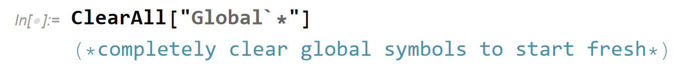
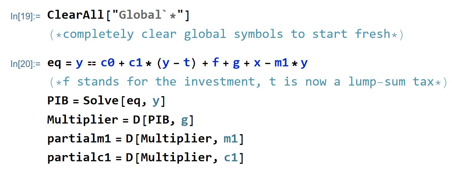
First, I have to clear the symbols to be sure that the previous registered symbol will not interfere with your model. Use (*something*) to insert the comment “something”:
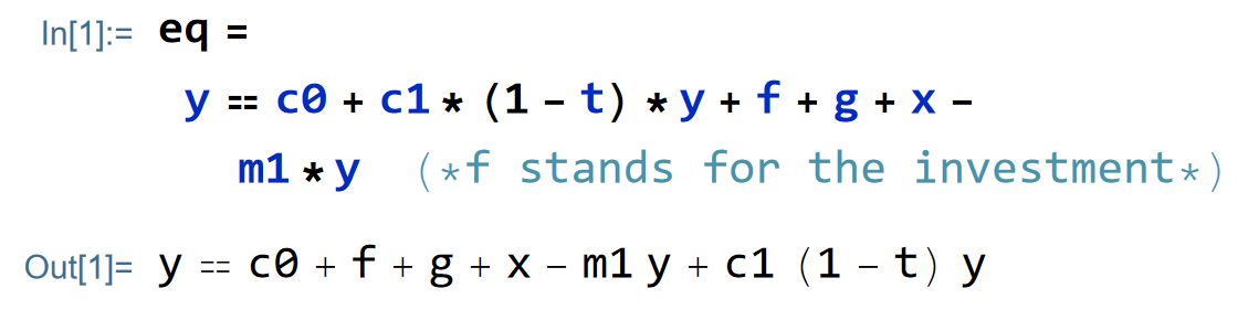
Then, I will use a first version of the model, with a tax rate. I name the equation ‘eq’ and I declare that my model can be reduced to one equation, where the GPD is in function of a consumption function, exogenous investment, exogenous government expenditures, exogenous exports, and an import function. I use ‘f’ for the investment to not confuse with imaginary numbers and for the french formation brute de capital fixe. You have to use Ctrl+Enter to execute the command. The above line gives this the following output:
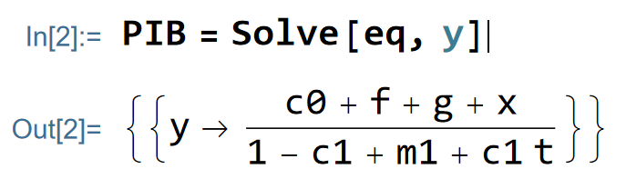
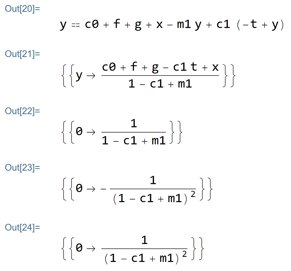
Then, I solve the model and I store the result in an object ‘PIB’ (the french acronym for GDP):
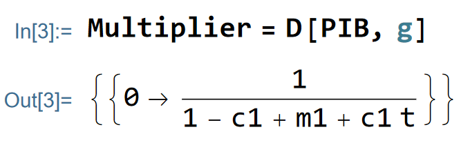
Now, I want to compute the algebraic value of the multiplier effect of this model. By definition, the multiplier is the value of a change in the GDP after an increase in an exogenous expenditure. In this example, I choose to evaluate the value of change in the GDP after an increase in exogenous government spending. I store the value in an object called ‘Multiplier’. The numerical value will depend on the value of the parameters of your models.
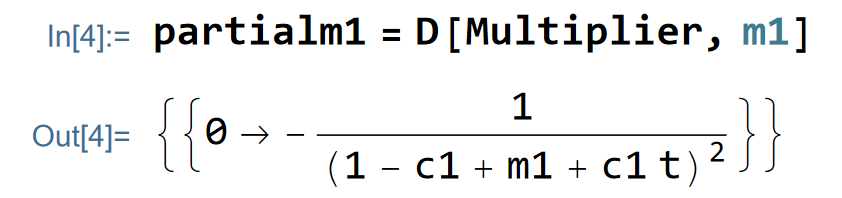
In the chapter 16 of the book, we can read that the multiplier is positively linked with the marginal propensity to consume and is negatively linked with the tax rate and the marginal propensity to import. I will derive the value of the multiplier relatively to these three last variables. The partial derivative of the multiplier effect relative to marginal propensity to import is indeed negative:
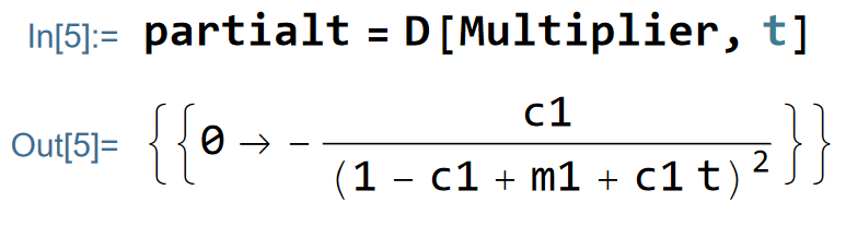
Besides, the partial derivative of the multiplier effect relative to the tax rate is also negative:
Finally, the partial derivative of the multiplier effect relative to the marginal propensity to consume is positive.
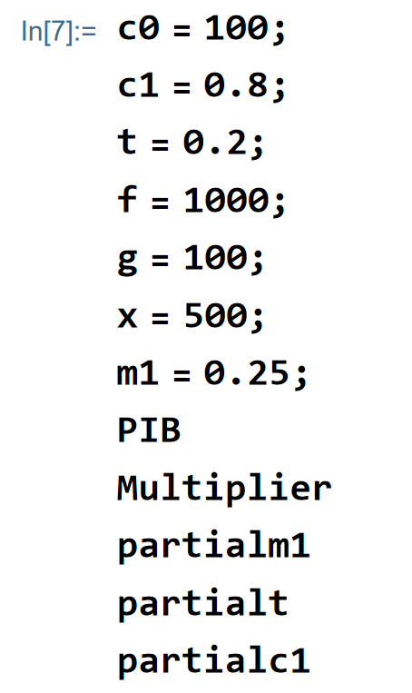
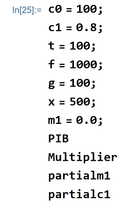
Now, we run a numerical example to determine (a) the equilibrium GDP, (b) the size of the multiplier effect, and (c) the sign of the partial derivatives by choosing vales for the exogenous variables and the parameters:
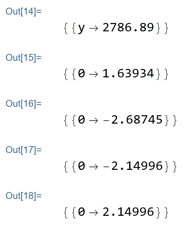
I use ‘;’ to hide the output. We found the equilibrium value for the GDP (2786.9), the size of the multiplier (1.63934), and the excepted signs for the partial derivative.
I can use a version of the model with lump-sum taxes to evaluate the balanced budget multiplier (a simultaneous and equivalent increase in public consumption and in taxes).
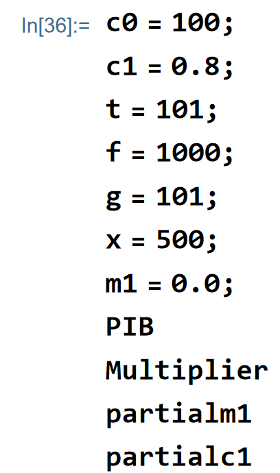
To simplify, I use a version of this model with lump-sum taxes where the propensity to import is equal to zero and evaluate the balanced budget multiplier:
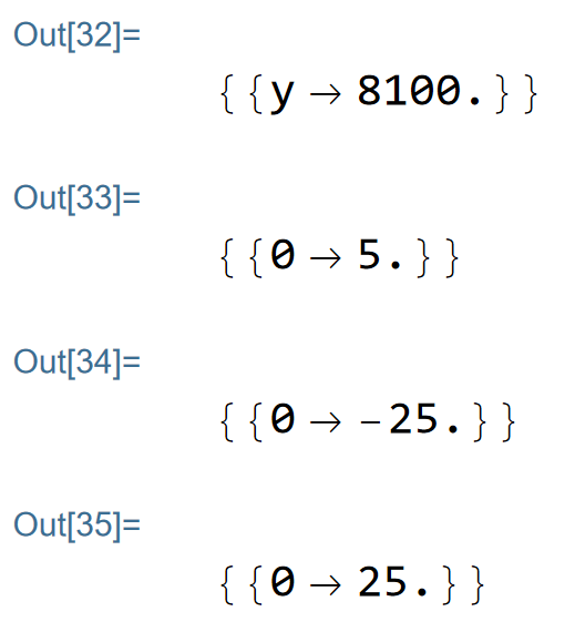
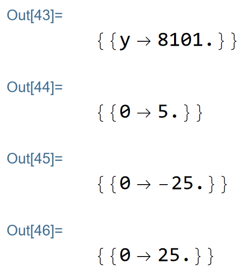
After an increase in public expenditures and in taxes, we can observe that the balanced budget multiplier is equal to one since the equilibrium GDP moves from 8100 to 8101 (‘g’ moved from 100 to 101 and ‘t’ moved from 100 to 101):
Reference
- Economics, Fourteenth Edition, Richard Lipsey and Alec Chrystal, 2020, ISBN: 9780198791034, 792 pages, https://global.oup.com/