Bayesian quantile regression

In the latest edition of the Stata News, I learned that Stata has adapted the Bayesian quantile estimator of Yu and Moyeed (2001). You need to have access to Stata Now to run this new command. In my last ADB Working Paper, written with Joshua Aizenman, Donghyun Park, Irfan A. Qureshi, and Gazi S. Uddin, we provide empirical evidence that “higher government stability provides a better resilience to depreciation for higher quantiles of the depreciation rate“. We arrived to this conclusion using the traditional frequentist methods for the quantile regressions.

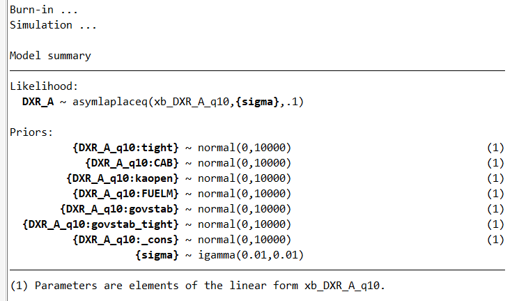
What will happen if I use the Yu and Moyeed’s estimator to consider uncertainty about the parameters? This estimator appears to be relevant since the sample size is limited in both the cross-sectional regressions and the “pseudo-panel” regression. Let me implement the command for the quantile 0.1 of the bilateral exchange rate (indirect quote for emerging markets) and, then, I will test whether the interaction term between the tightening dummy and the government stability variable (ICRG database, PRS group) is different for the quantile 0.9. The command is the following for the quantile 0.1:

#delimit ;
bayes, rseed(123): qreg    
          DXR_A tight CAB
          kaopen 
          FUELM 
          govstab govstab_tight
          if _est_stepwise_1==1, quantile(0.10);
#delimit cr

Yu and Moyeed (2001) mentioned that “Irrespective of the actual distribution of the data, Bayesian inference for quantile regression proceeds by forming the likelihood function based on the asymmetric Laplace distribution (Koenker and Bassett, 1978). In general, one may choose any prior, but we show that the use of improper uniform priors produces a proper joint posterior.” That is an attractive feature, as the choice of priors is an important question in Bayesian econometrics. We obtain the following results. The credible set of the interaction term ‘govstab_tight’ includes zero :

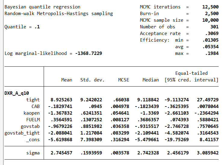
During a Stata webinar, Megan Cain (from Stata Corp) recalled me the difference for the interpretation between confidence intervals and credible intervals. For the confidence interval: with repeated sampling, if I fit my model in each of those samples and calculate the confidence interval, 95% of those confidence intervals will contain the true value. For the credible interval: There is a 95% probability the best value is in this interval. They both consider uncertainty in the parameters. In the Bayesian approach, we believe the parameters have a random distribution, however, whereas in the frequentist framework we believe there is one true population value. Now, I look at the quantile 0.9:

#delimit ;
bayes, rseed(123): qreg  
          DXR_A tight CAB
          kaopen 
	  FUELM 
          govstab govstab_tight
          if _est_stepwise_1==1, quantile(0.90);
#delimit cr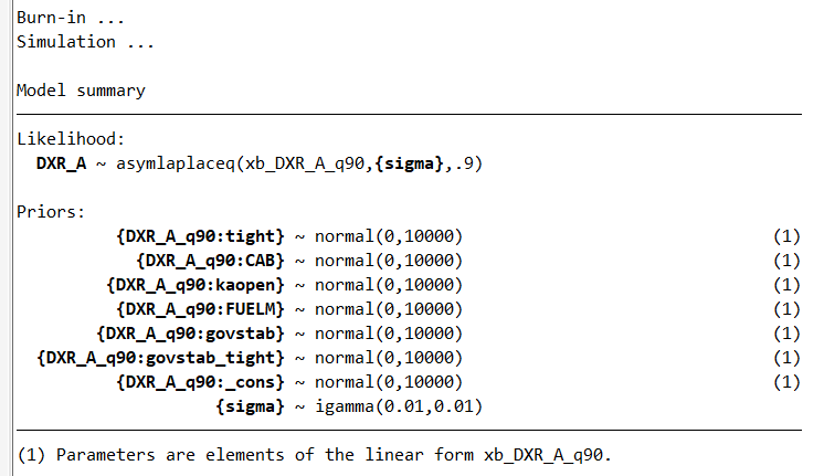

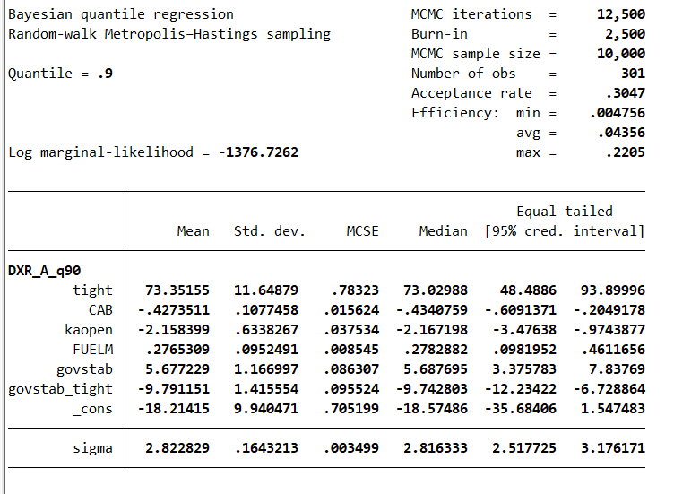
I can test the asymmetry between the quantile 0.1 and 0.9 thanks to the lower and upper bounds of the estimates for the quantile 0.1. The asymmetry is confirmed as the probability that the coefficient ‘govstab_tight’ lies between -4.582 and .316 is 0. Thus, we have further evidence showing that “Higher government stability provides a better resilience to depreciation for higher quantiles of the depreciation rate“, especially during tightening monetary cycles.

#delimit ;
bayestest interval {DXR_A_q90:govstab_tight},
 lower(-4.582) upper(.316);
#delimit cr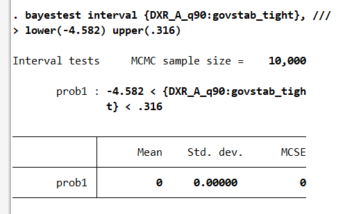

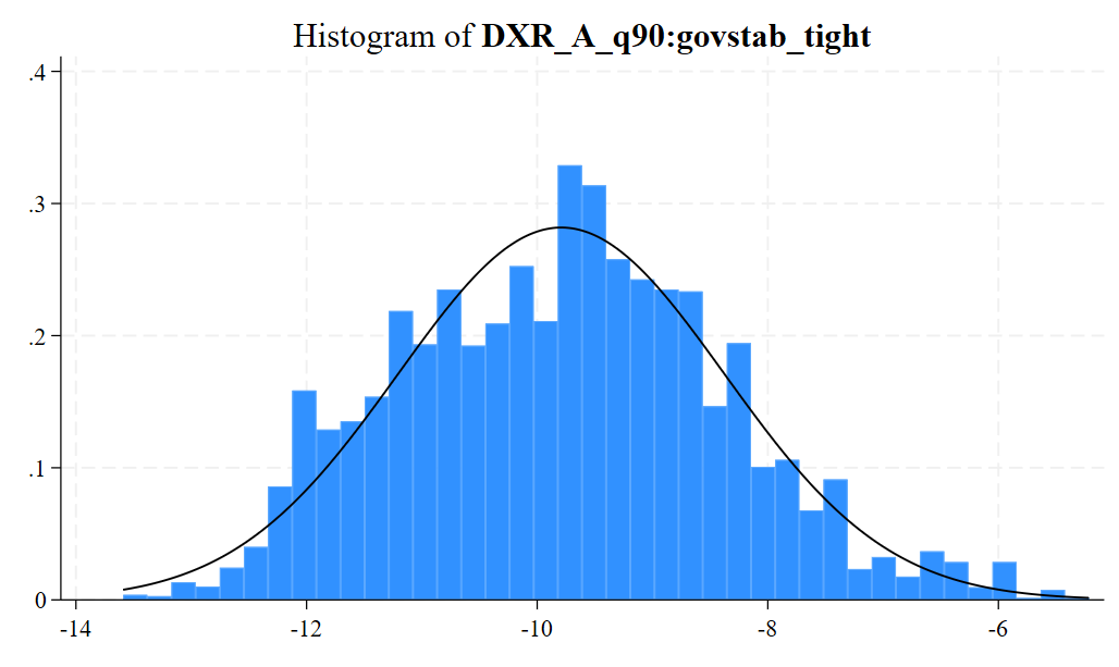
Finally, we can look at some diagnostic graphs for the interaction term by running the following command just after the estimation. The histogram shows that the parameter has a posterior distribution centered around -9.79 a value close to the value obtained for the quantile regression with the frequentist approach (-10.37):

#delimit ;
bayesgraph diagnostics {govstab_tight};
bayesgraph histogram {govstab_tight}, 
 normal;
#delimit cr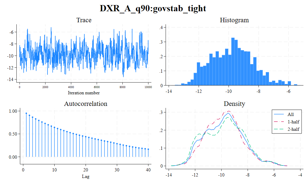

Reference

‌Aizenman, Joshua, Donghyun Park, Irfan A Qureshi, Jamel Saadaoui, and Gazi S Uddin (2024). “The Performance of Emerging Markets During the Fed’s Easing and Tightening Cycles: A Resilience Analysis Across Economies.” Asian Development Bank, August 14, 2024.

Yu, Keming, and Rana A Moyeed. 2001. “Bayesian Quantile Regression.” Statistics & Probability Letters 54 (4): 437–47. https://doi.org/10.1016/s0167-7152(01)00124-9.