Suppose that a rise in geopolitical risk does not have the same effect when a country begins in a tranquil environment and when tensions are already elevated. A hard state-dependent local projection assigns every observation to one regime or the other. A smooth-transition local projection asks a subtler question: can the conditional response change gradually as the initial environment changes?
1. Start from the linear local projection
At horizon \(h\), a conventional panel local projection estimates the future outcome directly:
\[ \mathrm{RATE}_{i,t+h} = \alpha_i^h + \beta_h \mathrm{GPR}_{i,t} + \boldsymbol{\Pi}_h^{\prime}\mathbf{X}_{i,t-1} + \rho_h\mathrm{REC}_{i,t} + u_{i,t+h}. \]Here \(\mathrm{RATE}_{i,t+h}\) is the short-term interest rate in economy \(i\), \(\mathrm{GPR}_{i,t}\) is current geopolitical risk, and \(\alpha_i^h\) denotes horizon-specific country fixed effects. The vector \(\mathbf{X}_{i,t-1}\) contains controls observed at \(t-1\) or earlier. The recession indicator is written separately as \(\mathrm{REC}_{i,t}\) because it is a contemporaneous channel control: the coefficient \(\beta_h\) traces the GPR response while holding the current recession channel fixed. Estimating one regression for each \(h\) gives the response path \(\{\beta_0,\ldots,\beta_H\}\).
\[ \mathbf{X}_{i,t-1} =\left( \mathrm{RATE}_{i,t-1},\mathrm{RATE}_{i,t-2}, \mathrm{GPR}_{i,t-1}, \mathrm{GAP}_{i,t-1},\mathrm{GAP}_{i,t-2}, \mathrm{INF}_{i,t-1},\mathrm{INF}_{i,t-2} \right)^{\prime}. \]The timing is therefore easy to read. Current GPR is the impulse variable, while the smooth state and ordinary macroeconomic controls are predetermined. This timing implements the recursive short-run restriction. Current recession status is the one contemporaneous channel control; including it does not assign recession a causal effect on GPR.
“estimated by simple regression techniques with standard regression packages”
Jordà (2005), American Economic Review
That flexibility is exactly why LPs accommodate nonlinear specifications so naturally. Jordà and Taylor (2025) later called the method a convenient and versatile tool in the empiricist’s kit
. The LP estimator does not choose the shock for us; the short-run restriction does. Entering current GPR while using lagged interest-rate, GPR, output-gap, and inflation controls allows those macroeconomic variables to react to GPR within month \(t\), while ruling out feedback from their date-\(t\) innovations into the GPR shock. Under that maintained restriction, \(\beta_h\) is the response to the recursively identified current-GPR innovation, conditional on current recession status.
“Local projections can have short-run restrictions because the restrictions define the shock, not the estimator.”
Earlier EconMacro note: Can Local Projections Have Short-Run Restrictions?
2. Why replace a hard regime?
A hard-state design might define a high-GPR observation as
\[ S_{i,t-1} = \mathbf{1}\!\left\{\mathrm{GPR}_{i,t-1}\gt P_{75,i}\right\}. \]Then the shock enters as \((1-S)\mathrm{GPR}\) and \(S\mathrm{GPR}\). This is transparent, and hard thresholds remain useful when the economic state is genuinely discrete. Yet the construction also creates a cliff: two almost identical observations can be placed in different regimes simply because one falls just below the cutoff and the other just above it.
What a smooth state gains
It avoids all-or-nothing assignment, uses observations on both sides of the midpoint, and makes the response a continuous function of the initial condition.
What a smooth state costs
It imposes a transition shape, requires a midpoint and steepness calibration, and can conceal weak support if researchers report only the limiting states.
“allowing these multipliers to vary smoothly according to the state of the economy”
Auerbach and Gorodnichenko (2013), Fiscal Multipliers in Recession and Expansion
“more of the observations are taken to contain some information about behaviour in both regimes”
Tenreyro and Thwaites (2016), American Economic Journal: Macroeconomics
This article follows that smooth-state intuition. It does not replicate the full Auerbach–Gorodnichenko design. The present model is deliberately parsimonious: the intercept and current-GPR slope vary with the state, while the lag and control coefficients remain common.
3. Build a country-relative smooth state
3.1 Standardize lagged GPR within each economy
\[ z_{i,t-1} = \frac{\mathrm{GPR}_{i,t-1}-\overline{\mathrm{GPR}}_{i,-1}} {s_{\mathrm{GPR},i,-1}}. \]The state is lagged, so it is known before the current GPR realization. The mean and standard deviation are economy-specific. Therefore, \(z=0\) means “equal to this economy’s own historical mean,” not “equal to the cross-country mean.” This prevents the state from becoming a disguised country label.
3.2 Map the standardized state into a weight
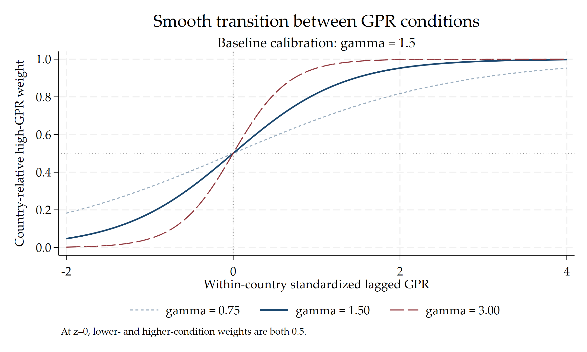
\[ F_{i,t-1} = \frac{1}{1+\exp\!\left[-\gamma\left(z_{i,t-1}-c\right)\right]}, \qquad 0\lt F_{i,t-1}\lt 1. \]The baseline sets the midpoint \(c=0\) and the steepness \(\gamma=1.5\). At the midpoint, \(F=0.5\). The slope of the logistic curve is \(\gamma F(1-F)\), so its maximum slope is \(\gamma/4\) at \(z=0\). A larger \(\gamma\) makes the transition more threshold-like; a smaller \(\gamma\) spreads the transition over a wider range of GPR. This logistic map comes from the broader smooth-transition time-series tradition formalized by Teräsvirta (1994); the LP literature adapts the idea to horizon-by-horizon projections.
3.3 Check support before estimating anything
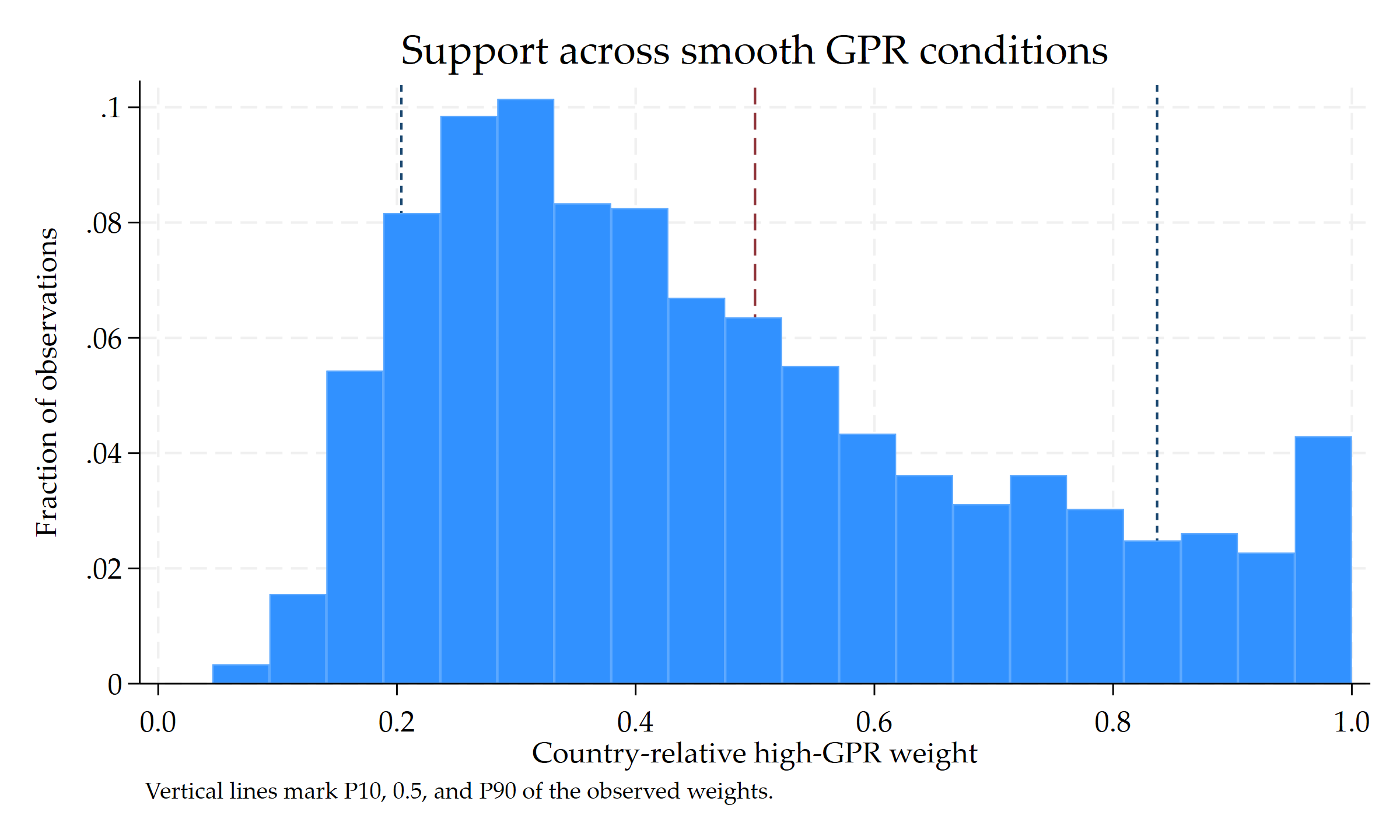
The developed-economy panel contains Canada, Denmark, the euro area, Japan, Norway, Sweden, Switzerland, the United Kingdom, and the United States: 2,385 monthly observations from February 2000 to February 2022. Lagging GPR leaves 2,376 state observations. All nine economies are observed on both sides of \(F=0.5\).
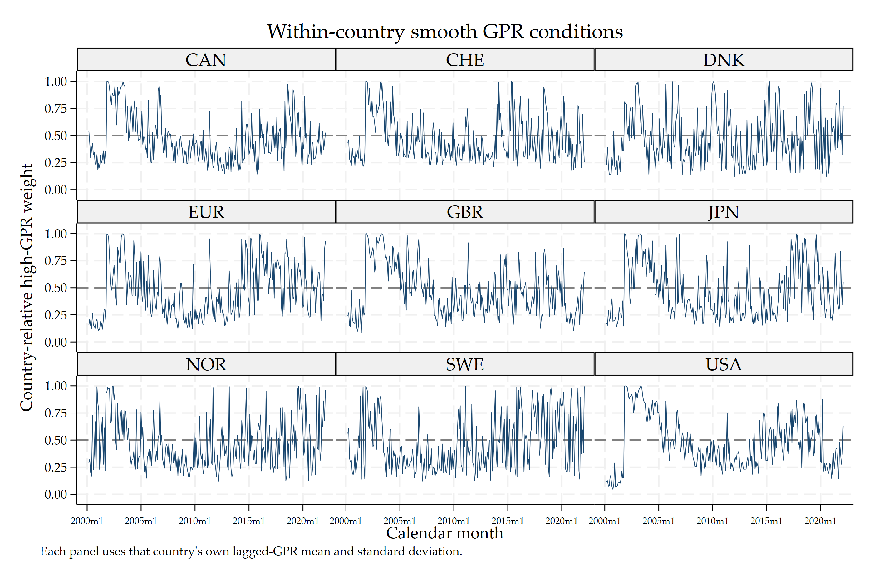
| Calibration | P10(F) | P90(F) | P90−P10 | Interpretation |
|---|---|---|---|---|
| \(\gamma=0.75\) | 0.3359 | 0.6937 | 0.3578 | Gentle transition |
| \(\gamma=1.50\) | 0.2037 | 0.8369 | 0.6332 | Baseline |
| \(\gamma=3.00\) | 0.0614 | 0.9634 | 0.9020 | Steep transition |
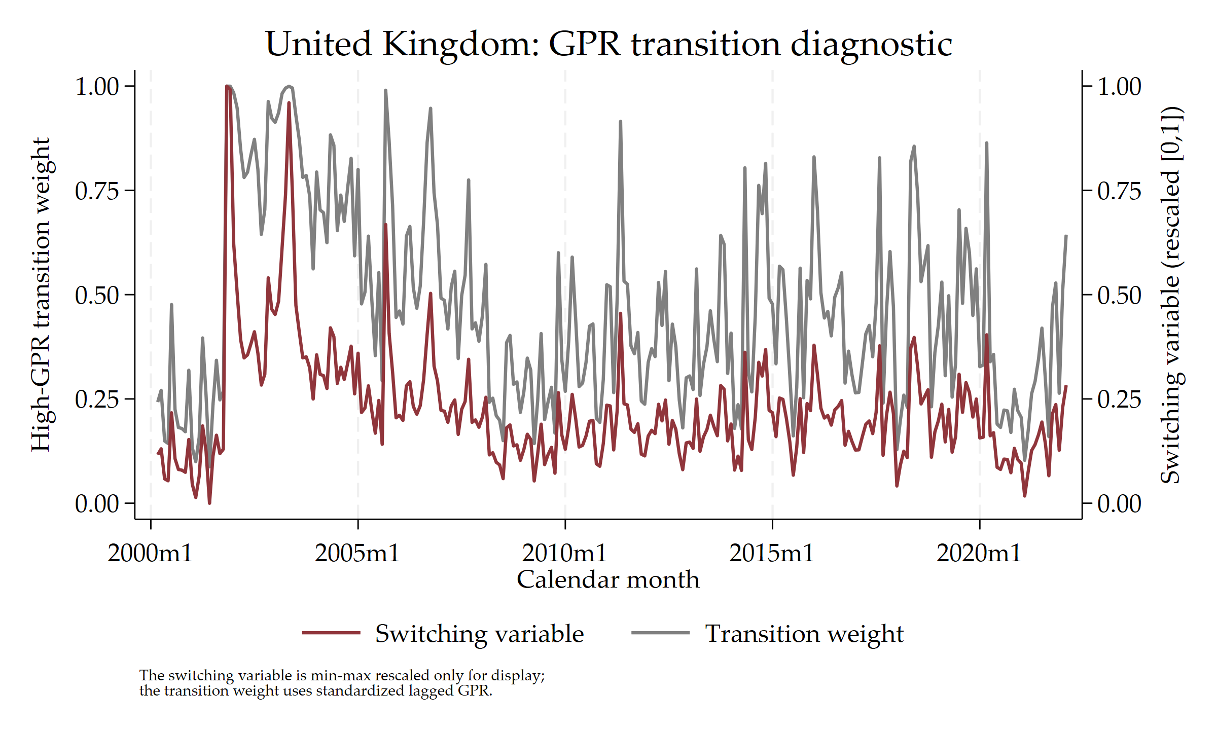
3.4 Read the UK diagnostic correctly
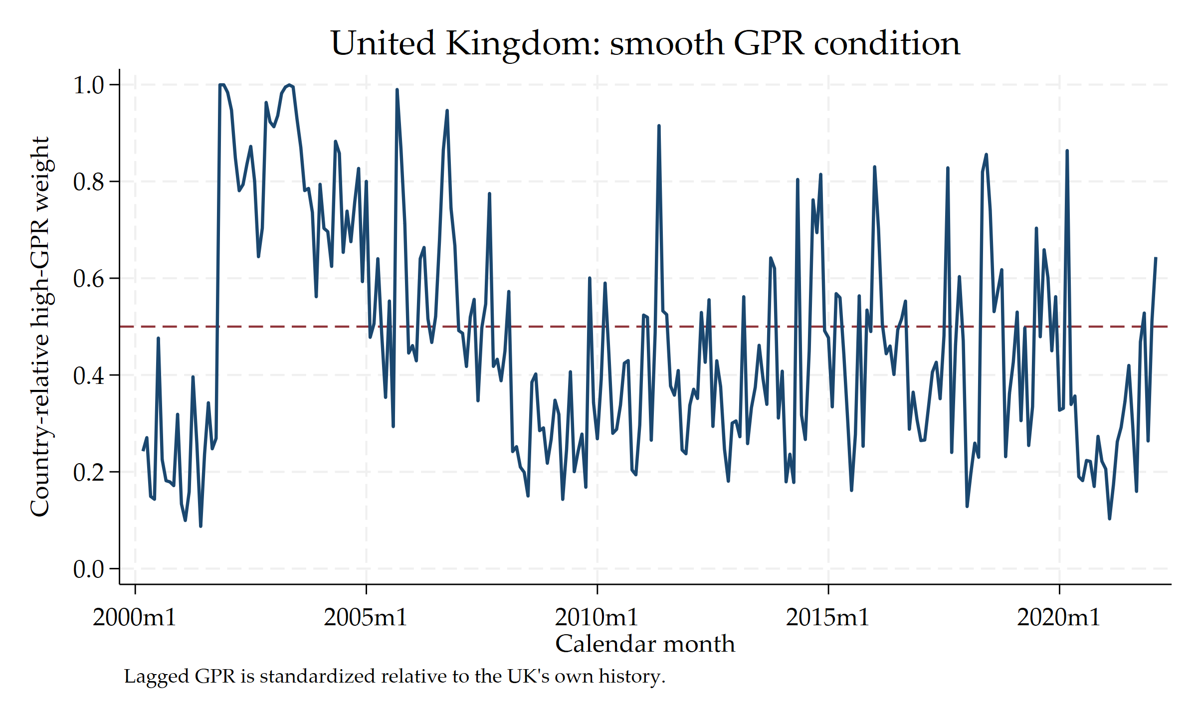
The dashed line at 0.5 is especially useful. Crossing it means that lagged GPR crosses the within-UK mean. It does not mean that the economy suddenly enters a different data-generating process. That distinction is the whole point of the smooth specification.
The next graph is a coding diagnostic. Its red series min–max rescales the standardized lagged-GPR switching variable to the interval from zero to one solely so that it can share an axis with the logistic weight. The blue series applies the logistic formula to that standardized state. The two transformations are monotonic, but only the blue series is the weight used in the regressions. Neither line is a probability of conflict.
4. Define the estimand before reading the graph
4.1 Split current GPR exactly
\[ \begin{aligned} \mathrm{GPR}_{i,t}^{L} &= \left(1-F_{i,t-1}\right)\mathrm{GPR}_{i,t},\\ \mathrm{GPR}_{i,t}^{H} &= F_{i,t-1}\mathrm{GPR}_{i,t},\\ \mathrm{GPR}_{i,t}^{L}+\mathrm{GPR}_{i,t}^{H} &= \mathrm{GPR}_{i,t}. \end{aligned} \]Nothing is thrown away. Every current-GPR observation enters both components. Only its relative contribution changes with the lagged state.
4.2 Estimate a restricted varying-coefficient LP
\[ \begin{aligned} \mathrm{RATE}_{i,t+h} &= \alpha_i^h+\delta_hF_{i,t-1}\\ &\quad +\beta_h^L\left(1-F_{i,t-1}\right)\mathrm{GPR}_{i,t} +\beta_h^HF_{i,t-1}\mathrm{GPR}_{i,t}\\ &\quad +\boldsymbol{\Pi}_h^{\prime}\mathbf{X}_{i,t-1} +\rho_h\mathrm{REC}_{i,t} +u_{i,t+h}. \end{aligned} \]The lagged control vector contains two lags of the interest rate, one lag of GPR, two lags of the output gap, and two lags of inflation. Contemporaneous recession status enters separately through \(\rho_h\mathrm{REC}_{i,t}\) to hold the recession channel fixed. It is not included because recession is assumed to cause GPR. The model includes country fixed effects and no time fixed effects. The coefficient \(\delta_h\) lets the conditional intercept shift with the state; the two \(\beta\) coefficients let the current-GPR slope vary.
“We allow all of the coefficients of the model to vary according to the state of the economy.”
Ramey and Zubairy (2018), Journal of Political Economy
That quotation clarifies the restriction in the present exercise. A canonical fully state-dependent specification interacts the state with the constant, shock, and conditioning variables. Here the state intercept and current-GPR slope vary, but the lag and control slopes are held common. I therefore interpret this as a parsimonious varying-GPR-slope LP, inspired by the smooth-transition literature rather than a full replication of its conditional mean.
4.3 Endpoint coefficients are not observed regimes
At any chosen weight \(f\), the conditional projection slope is
\[ R_h(f)=(1-f)\beta_h^L+f\beta_h^H. \]For compactness, \(R_h(f)\) suppresses the conditioning on \(\mathrm{REC}_{i,t}\). Throughout the article, recession status is held fixed, so this is the GPR response net of the contemporaneous recession channel.
\(\beta_h^L\) and \(\beta_h^H\) describe the limiting endpoints \(F=0\) and \(F=1\). Finite values of the logistic index do not reach those endpoints exactly. Calling the endpoint coefficients “the low regime” and “the high regime” would therefore overstate the empirical support.
The code instead evaluates two interior paths:
\[ \begin{aligned} R_h(F_{10}) &=0.7963\beta_h^L+0.2037\beta_h^H,\\ R_h(F_{90}) &=0.1631\beta_h^L+0.8369\beta_h^H. \end{aligned} \]The supported higher-minus-lower contrast is
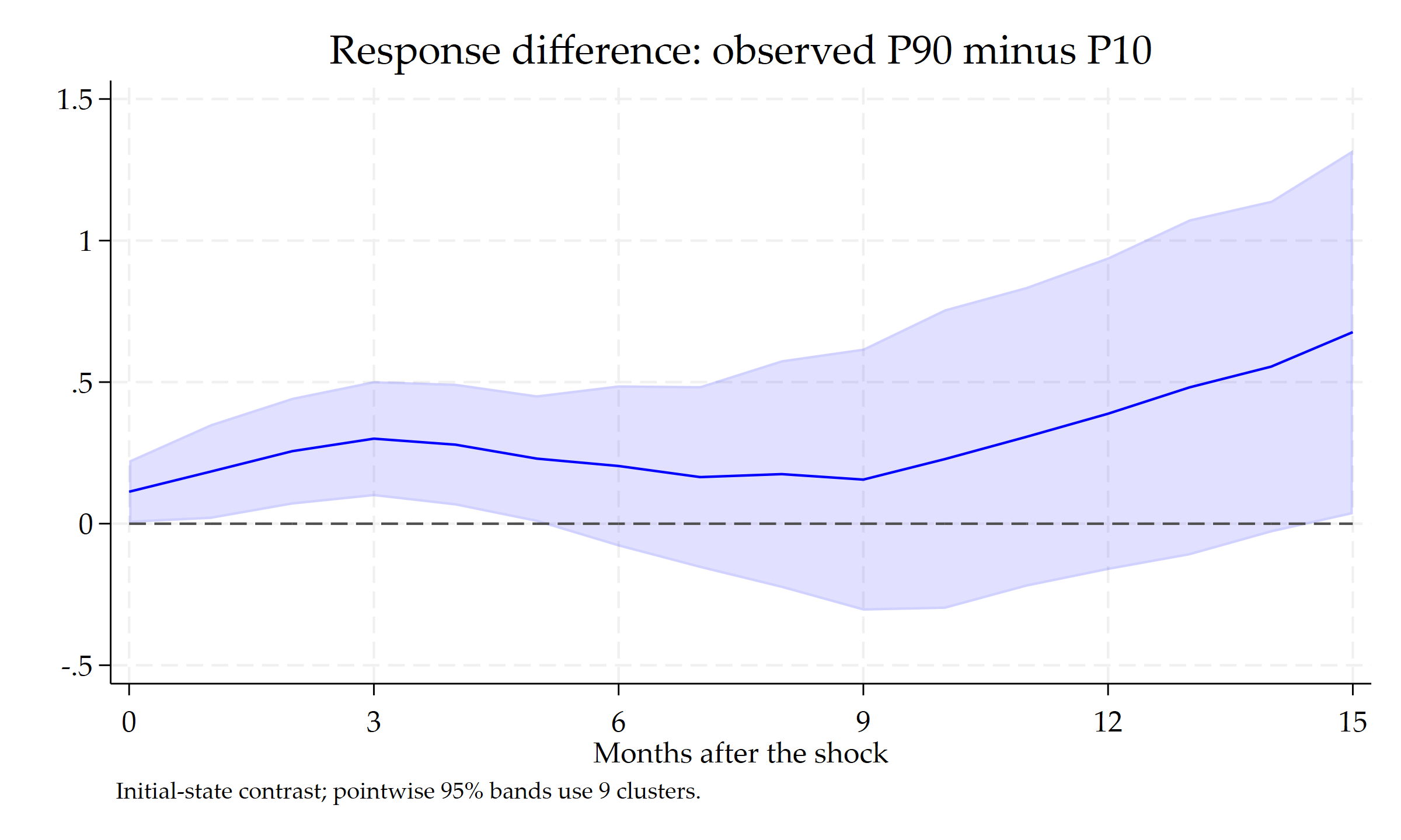
\[ \Delta_h^{90-10} =(F_{90}-F_{10})(\beta_h^H-\beta_h^L) =0.6332(\beta_h^H-\beta_h^L). \]This is why the reported contrast is not simply \(\beta_h^H-\beta_h^L\). The latter is an endpoint contrast; the former compares two states that are actually supported by the data.
“users need to be explicit about which population response they are interested in recovering”
Gonçalves, Herrera, Kilian, and Pesavento (2024), Journal of Econometrics
Their result matters here. If the state responds endogenously to macroeconomic shocks, a conventional state-dependent LP generally has a clean interpretation for an infinitesimal conditional response only under additional assumptions; it need not recover the nonlinear response to a large shock. The present application therefore reports a recursively identified response conditional on the initial state. For a large shock, it should not automatically be read as the response associated with a permanently fixed regime.
5. Translate the algebra into Stata—without local macros
5.1 Construct the state and the two GPR components
* Predetermined state: GPR at t-1
generate double gpr_l1 = L.gpr

* Country-relative standardization
bysort imfcode: egen double mean_gpr_l1 = mean(gpr_l1)
bysort imfcode: egen double sd_gpr_l1   = sd(gpr_l1)
generate double z_gpr_l1 = ///
    (gpr_l1-mean_gpr_l1)/sd_gpr_l1 if !missing(gpr_l1)

* Baseline logistic weight
scalar stlp_gamma = 1.5
generate double st_weight = ///
    invlogit(scalar(stlp_gamma)*z_gpr_l1) if !missing(z_gpr_l1)

* Exact decomposition of current GPR
generate double gpr_low_st  = (1-st_weight)*gpr
generate double gpr_high_st = st_weight*gpr

assert abs(gpr_low_st+gpr_high_st-gpr)<1e-10 ///
    if !missing(st_weight,gpr)
The final assertion is more than housekeeping. It proves that the two regressors are an exact state-weighted decomposition of the original current-GPR variable.
5.2 Compute supported evaluation weights
summarize st_weight, detail
scalar stlp_f10    = r(p10)
scalar stlp_f90    = r(p90)
scalar stlp_omf10 = 1-scalar(stlp_f10)
scalar stlp_omf90 = 1-scalar(stlp_f90)
scalar stlp_fgap  = scalar(stlp_f90)-scalar(stlp_f10)
These percentiles are sample-specific and observation-weighted. They are not universal definitions of low and high geopolitical risk.
5.3 Ask locproj for the P10 path
locproj RATE, ///
    shock(gpr_low_st gpr_high_st) ///
    lcs(gpr_low_st*stlp_omf10+gpr_high_st*stlp_f10) ///
    zero h(0/15) yl(2) ///
    c(st_weight L.gpr L(1/2).impact_gap L(1/2).INF rec) ///
    fe cluster(imfcode) conf(95) ///
    saveirf irfname(D2S1_st_p10) noisily stats ///
    grname(D2S1_st_p10)
The time operators implement the equation directly. yl(2) adds \(\mathrm{RATE}_{i,t-1}\) and \(\mathrm{RATE}_{i,t-2}\); L.gpr is dated \(t-1\); and L(1/2) adds the first two lags of the output gap and inflation. This lag structure implements the recursive short-run restriction. The variables st_weight and rec appear without an L. prefix for different reasons: st_weight is already constructed from L.gpr, whereas rec is intentionally contemporaneous so that the reported GPR response is net of the current recession channel.
| Option | What it does | Economic meaning |
|---|---|---|
shock(...) |
Estimates both weighted GPR slopes jointly. | One regression contains the low- and high-condition components. |
lcs(...) |
Forms the requested linear combination. | Evaluates the response at the observed P10 weight. |
h(0/15) |
Estimates impact through month 15. | Sixteen direct horizon regressions. |
yl(2) |
Adds two outcome lags. | Controls for interest-rate dynamics. |
c(...) |
Adds the predetermined state, lagged macro controls, and current recession status. | The lagged macro controls implement the short-run restriction; current recession status separately holds the recession channel fixed. |
fe cluster(imfcode) |
Adds country fixed effects and country-clustered inference. | Uses within-country identifying variation, with the few-cluster caution discussed below. |
5.4 Estimate the contrast directly
locproj RATE, ///
    shock(gpr_low_st gpr_high_st) ///
    lcs(gpr_high_st*stlp_fgap-gpr_low_st*stlp_fgap) ///
    zero h(0/15) yl(2) ///
    c(st_weight L.gpr L(1/2).impact_gap L(1/2).INF rec) ///
    fe cluster(imfcode) conf(95) ///
    saveirf irfname(D2S1_st_diff) noisily stats ///
    grname(D2S1_st_diff)
Estimating the contrast directly preserves the covariance between the two slope estimates. For constants \(a\) and \(b\),
\[ \operatorname{SE}\!\left( a\widehat{\beta}_h^L+b\widehat{\beta}_h^H \right) = \left[ a^2\operatorname{Var}\!\left(\widehat{\beta}_h^L\right) +b^2\operatorname{Var}\!\left(\widehat{\beta}_h^H\right) +2ab\operatorname{Cov}\!\left( \widehat{\beta}_h^L,\widehat{\beta}_h^H \right) \right]^{1/2}. \]Comparing whether two separate confidence bands overlap is not the same statistical test. This is the smooth-state analogue of the direct regime-comparison logic in Statistical Difference between Regimes in State-Dependent Local Projections using LOCPROJ.
The complete no-locals do-file is reproduced in Section 11.
6. Read the empirical estimates—but scale them first
The plotted response is for a one-unit recursively identified current-GPR innovation, measured in the original GPR units. The observed GPR index has a pooled standard deviation of 0.3912, so one index unit is about 2.56 standard deviations of the observed series. To report a 0.3912-unit innovation—a change equal in size to one pooled standard deviation of the observed GPR index—multiply every estimate and confidence limit by 0.3912. This is an observed-index normalization; it is not a claim that 0.3912 is the standard deviation of the residualized structural innovation.
\[ R_h^{0.3912\,\mathrm{GPR\ units}}(f) =0.3912\times R_h^{\text{one GPR-index unit}}(f). \]Every path below conditions on \(\mathrm{REC}_{i,t}\). The figures therefore show the recursively identified GPR response net of the contemporaneous recession channel, not a claim that recession causes GPR.
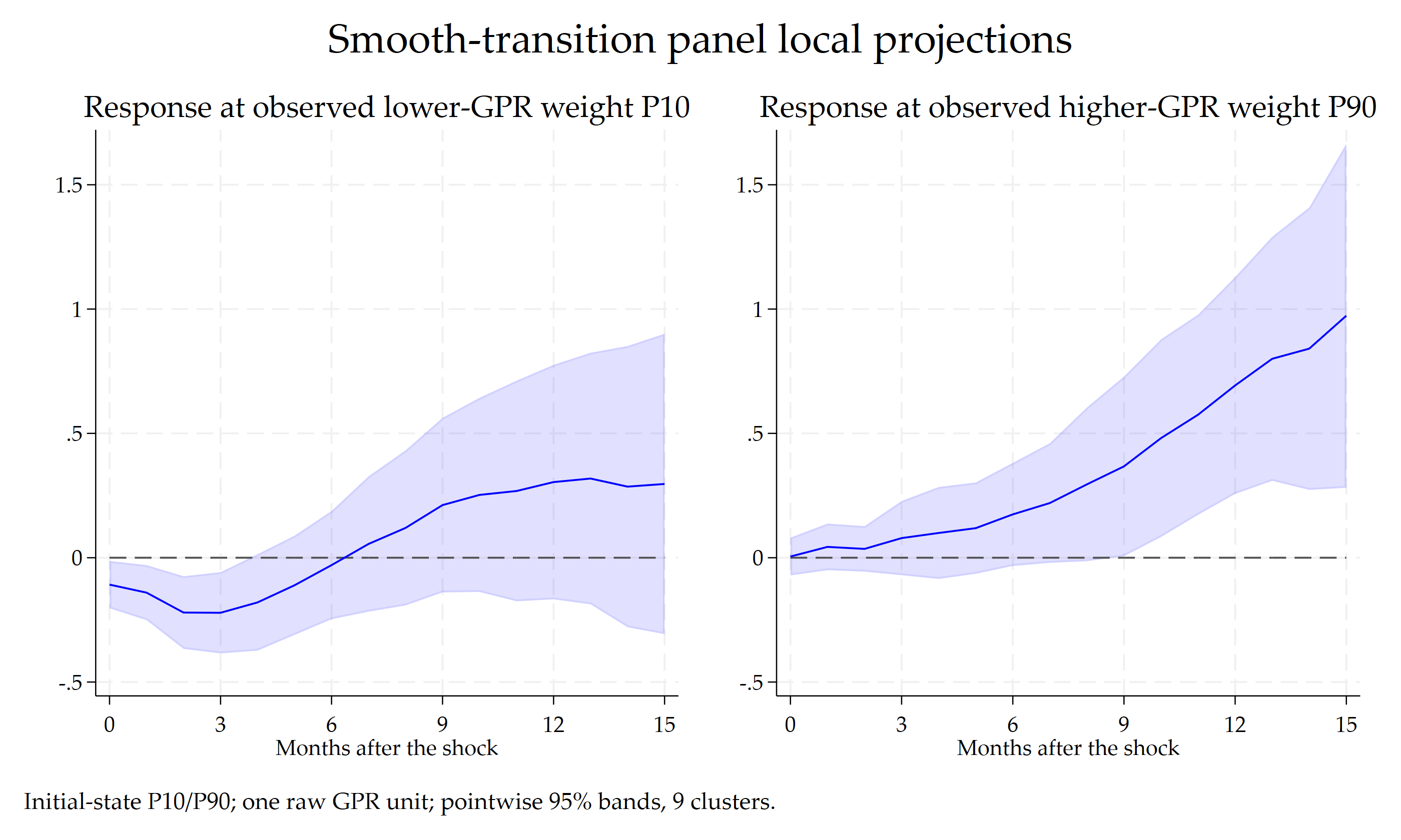
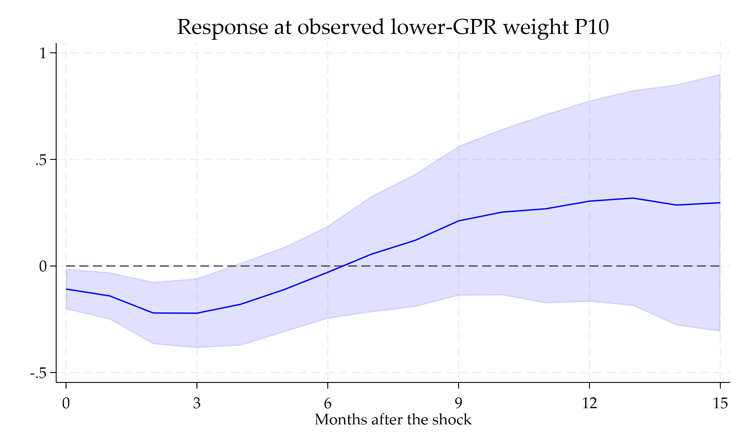
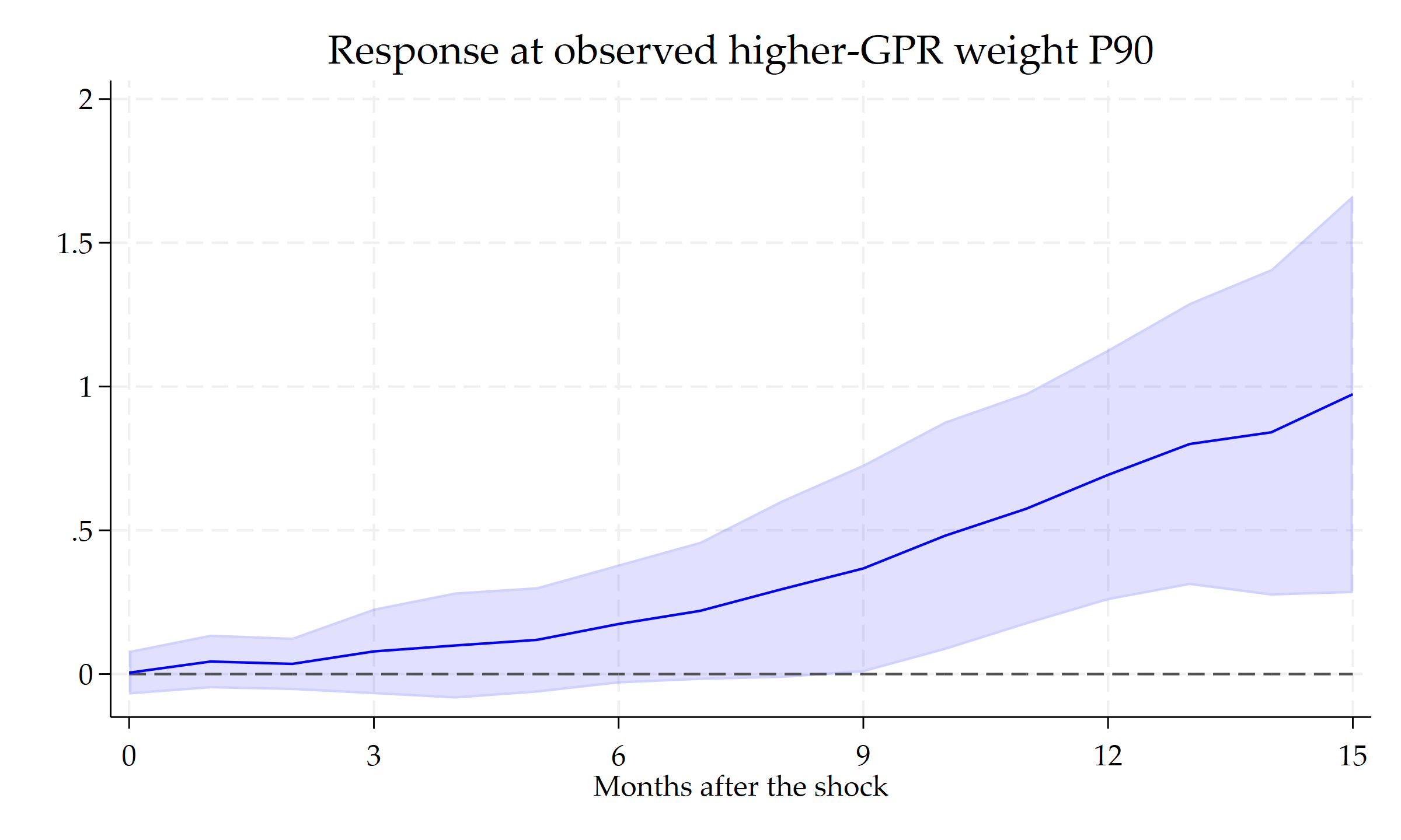
The combined graph makes the comparison easy; the two panels below make the uncertainty around each supported response easier to read.
| Month h | Lower-GPR P10 [95% CI] | Higher-GPR P90 [95% CI] | P90−P10 [95% CI] |
|---|---|---|---|
| 0 | −0.108 [−0.203, −0.013] | 0.005 [−0.071, 0.081] | 0.113 [0.003, 0.223] |
| 3 | −0.221 [−0.385, −0.058] | 0.079 [−0.070, 0.228] | 0.300 [0.097, 0.504] |
| 5 | −0.111 [−0.310, 0.089] | 0.119 [−0.065, 0.303] | 0.230 [0.006, 0.454] |
| 9 | 0.212 [−0.139, 0.563] | 0.367 [0.006, 0.729] | 0.156 [−0.307, 0.619] |
| 15 | 0.297 [−0.307, 0.901] | 0.973 [0.281, 1.665] | 0.677 [0.034, 1.320] |
Under the baseline calibration, the lower-GPR path is negative and pointwise significant from impact through month 3. The higher-GPR path becomes positive and pointwise significant from month 9 through month 15. The direct higher-minus-lower contrast is positive at every horizon, but its pointwise interval excludes zero only from month 0 through month 5 and again at month 15.
A concrete scaling example helps. At month 3, the one-unit estimates are −0.221 percentage point at P10 and 0.079 at P90, a difference of 0.300. For a 0.3912-unit innovation—equal in magnitude to one pooled standard deviation of the observed GPR index—these become approximately −0.087, 0.031, and 0.117 percentage point.
7. Treat \(\gamma\) as a calibration, not decoration
Changing \(\gamma\) does more than redraw the transition curve. It changes the weighted regressors, the empirical P10/P90 gap, and therefore the estimated coefficients and the estimand. The sensitivity exercise is central, not optional.
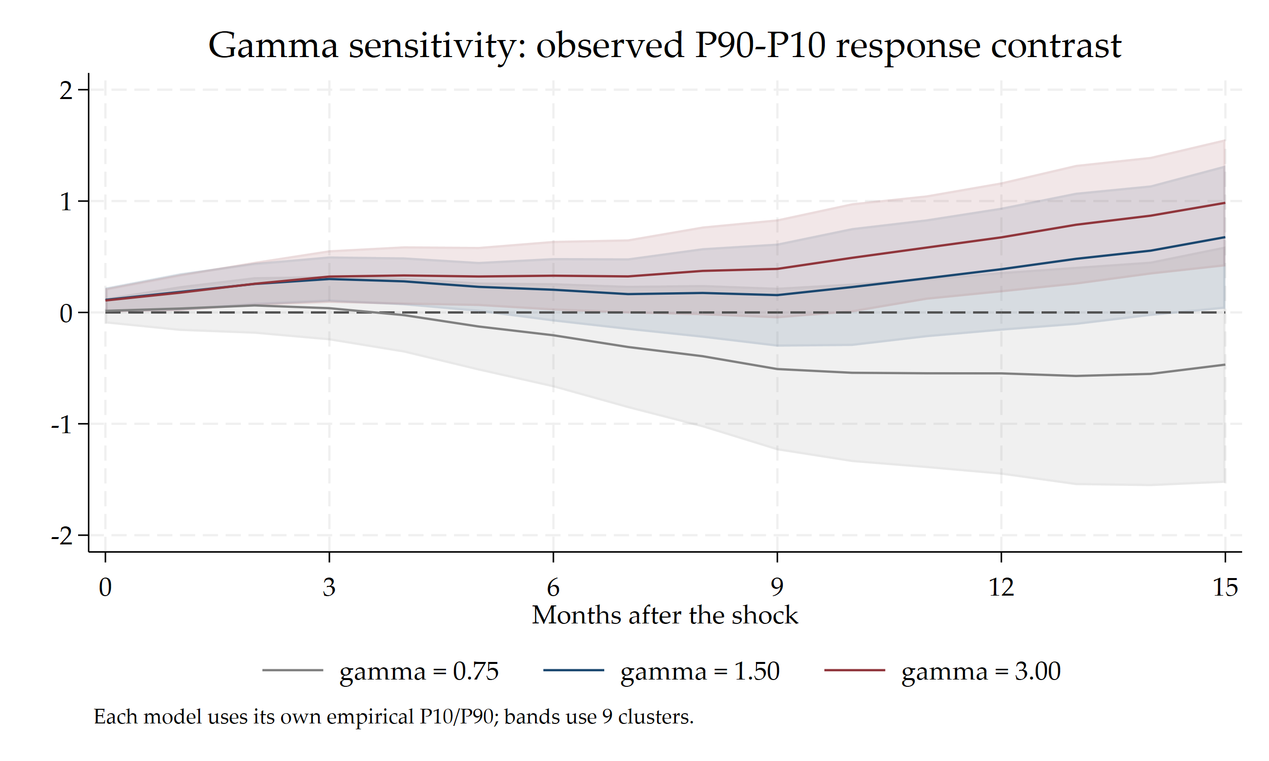
| Month h | \(\gamma=0.75\) [95% CI] | \(\gamma=1.50\) [95% CI] | \(\gamma=3.00\) [95% CI] |
|---|---|---|---|
| 0 | 0.015 [−0.099, 0.128] | 0.113 [0.003, 0.223] | 0.108 [−0.000, 0.215] |
| 3 | 0.038 [−0.251, 0.327] | 0.300 [0.097, 0.504] | 0.322 [0.086, 0.559] |
| 9 | −0.508 [−1.238, 0.222] | 0.156 [−0.307, 0.619] | 0.391 [−0.053, 0.836] |
| 15 | −0.468 [−1.529, 0.593] | 0.677 [0.034, 1.320] | 0.985 [0.414, 1.555] |
With \(\gamma=0.75\), none of the contrasts is pointwise significant, and the point estimates turn negative after month 3. This prevents a calibration-invariant headline such as “high initial GPR always amplifies the interest-rate response.” The defensible conclusion is narrower: the baseline and steep transitions suggest positive state dependence, but the result is sensitive to how gradually the state is allowed to change.
A stronger research design would justify \(\gamma\) economically, estimate the transition parameters under an explicit criterion, or report a dense calibration grid. It could also vary the midpoint \(c\). The current \(c=0\) design asks whether transmission varies around each economy’s own historical mean; it is not a smooth replica of a P75 threshold.
8. Separate identification, estimation, and inference
These three questions are often blended together. They should not be.
| Question | What the code does | What remains |
|---|---|---|
| Identification: Which short-run ordering defines the shock? | Implements recursive identification by entering GPR at \(t\) while dating the state and ordinary macro controls at \(t-1\) or earlier. Current recession status is included separately as a channel control. | The causal interpretation is conditional on the maintained short-run restriction and information set. Including \(\mathrm{REC}_{i,t}\) changes the estimand; it does not assert that recession causes GPR. |
| Estimation: How can propagation vary? | Uses a logistic weight and estimates each horizon directly with locproj. |
The model restricts lag and control dynamics to be common across states and reports responses conditional on the initial state and net of the contemporaneous recession channel. |
| Inference: How uncertain is the path? | Reports country-clustered, pointwise 95% intervals. | There are only nine clusters; common global shocks may create cross-sectional dependence; \(\gamma\), the state moments, and P10/P90 are treated as fixed. |
8.1 How the LP implements the recursive short-run restriction
The timing convention is the identification design. The state and the ordinary macroeconomic controls are known at \(t-1\). Current GPR is placed before the current interest rate, output gap, and inflation in the recursive ordering. Those macroeconomic variables may respond to GPR within month \(t\), but their own date-\(t\) innovations are restricted from feeding back into the GPR shock within that same month:
\[ \mathrm{GPR}_{i,t} \ \prec\ \left( \mathrm{RATE}_{i,t}, \mathrm{GAP}_{i,t}, \mathrm{INF}_{i,t} \right), \]where \(\prec\) means “ordered before on impact.” Notice that \(\mathrm{REC}_{i,t}\) is not in this ordering statement. It enters the outcome equation to control a channel, not to define the GPR shock and not to claim that recession causes GPR. Under the maintained GPR-first restriction relative to the ordinary macroeconomic outcomes, current GPR is recursively identified; a separate LP-IV first stage is not required.
The Frisch–Waugh–Lovell theorem makes the regression implementation transparent. Let the full set of variables partialled out by the STLP be
\[ \mathbf{C}_{i,t} =\left( F_{i,t-1}, \mathbf{X}_{i,t-1}^{\prime}, \mathrm{REC}_{i,t}, \mathbf{D}_i^{\prime} \right)^{\prime}. \]Here \(\mathbf{D}_i\) denotes the country fixed-effect indicators. The command jointly residualizes the two columns \(\left(1-F_{i,t-1}\right)\mathrm{GPR}_{i,t}\) and \(F_{i,t-1}\mathrm{GPR}_{i,t}\) against \(\mathbf{C}_{i,t}\). That is a partial-regression operation, not a causal arrow from every control to GPR. The lagged elements of \(\mathbf{X}_{i,t-1}\) implement the short-run restriction; including \(\mathrm{REC}_{i,t}\) ensures that the estimated slopes compare current-GPR movements while holding the contemporaneous recession channel fixed. Given the maintained common-control specification, the two state-weighted terms are identified by the same recursive timing restriction.
“VAR-based structural identification—including short-run, long-run, or sign restrictions—can equivalently be performed using LPs, and vice versa.”
Plagborg-Møller and Wolf (2021), Econometrica
This is exactly the logic developed in Can Local Projections Have Short-Run Restrictions?: an LP can use the same recursive restriction as a VAR either by constructing the Cholesky innovation first or by choosing the timing of the shock and macro controls consistently. The present specification uses the latter route. The external-instrument strategy discussed in Geopolitical Turning Points and Macroeconomic Volatility is an alternative identification design and a possible robustness exercise—not a missing prerequisite for this LP.
“a news-based measure of adverse geopolitical events and associated risks”
Caldara and Iacoviello (2022), American Economic Review
The GPR index supplies the observable impulse variable; the lag timing supplies its recursive structural interpretation. Identification is therefore present, but it is conditional on the stated short-run restriction rather than assumption-free.
8.2 What current recession status changes: the estimand
The workshop specification keeps rec at date \(t\) to control the contemporaneous recession channel. This choice changes what the reported response means. At an initial state \(f\), the estimand is
In words, adding \(\mathrm{REC}_{i,t}\) reports the GPR response net of the contemporaneous recession channel. It compares observations with the same current recession status. This is why \(\mathrm{REC}_{i,t}\) is written separately from the predetermined vector \(\mathbf{X}_{i,t-1}\). The regression does not say that recession causes GPR; a conditioning variable is not automatically a causal parent of the impulse variable.
This channel-net response is different from the total response that would allow current GPR to operate through every contemporaneous change in recession status. Omitting current recession status, or replacing it with \(\mathrm{REC}_{i,t-1}\), would answer a different question and would require re-estimating the paths. The baseline here deliberately keeps \(\mathrm{REC}_{i,t}\) because the desired estimand excludes that contemporaneous recession channel.
8.3 Nine clusters are a warning, not a footnote
The panel is long—265 months per economy—but has only nine country clusters. The log correctly warns that conventional cluster-robust inference is fragile. In addition, global monetary and geopolitical shocks can correlate residuals across economies. Useful robustness checks include a wild-cluster bootstrap, leave-one-economy-out estimates, time fixed effects where the identifying variation permits them, and Driscoll–Kraay inference. The latter is illustrated in Drawing Local Projection IRFs with Driscoll–Kraay Inference in Stata.
Because the specification is dynamic and uses fixed effects, a publication exercise should also discuss finite-\(T\) bias. Here \(T\) is large, so the classic Nickell concern is less acute than in short panels, but it is still conceptually relevant; see Beware of the Nickell Bias if You Use Panel Local Projections.
8.4 Smooth state dependence does not repair other LP misspecification
The transition function answers a heterogeneity question. It does not prevent later shocks from contaminating horizon-specific projections. That separate issue is discussed in Adding Forward Shocks to Solve Misspecification in Local Projections with LOCPROJ. Likewise, smooth weighting does not remove persistence. The lag-augmentation logic developed in Thou Shalt Lag-Augment, Not “Stationarize” when Using Local Projections is important background, but its formal result is for time-series LPs and should not be presented as an automatic theorem for this panel STLP.
9. Do not confuse two meanings of “smooth”
Smooth-transition LP in this post
Smoothness is across the state. The weight \(F(z)\) changes continuously with lagged GPR. Horizon coefficients are still estimated separately.
Smooth local projections
Barnichon and Brownlees (2019) impose B-spline smoothness across the horizon to reduce variance. Their method preserves the flexibility of standard LP
while regularizing the response shape.
The two ideas can, in principle, be combined: a response could vary smoothly with the initial state and also be regularized across horizons. But they solve different problems. The current article uses smooth state weights and ordinary horizon-by-horizon LP estimation.
10. What the exercise establishes—and what it does not
What the exercise establishes
- The lag structure implements an explicit recursive short-run ordering for the GPR innovation.
- Current recession status is held fixed, so the estimand is net of the contemporaneous recession channel.
- All nine economies cross the midpoint.
- P10 and P90 evaluate the response inside the observed support.
- The contrast is estimated directly with its covariance.
- Gamma sensitivity is reported rather than hidden.
- The baseline recursively identified response differs across initial GPR conditions at several horizons.
- The state is predetermined and country-relative.
Robustness checks and research extensions
- Defend the recursive timing restriction economically and compare, when useful, with a specification that includes the contemporaneous recession channel.
- Justify or estimate \(\gamma\) and the midpoint, and report a broader calibration grid.
- Add few-cluster and cross-sectional-dependence robustness.
- Use simultaneous bands or joint path tests.
- Distinguish a raw-index normalization from normalization by the standard deviation of the residualized innovation.
- Test whether results survive time effects, leave-one-out samples, and alternative control timing.
- Use pre-sample or expanding-window state normalization if a real-time interpretation is intended.
11. Complete Stata code
The block below reproduces the complete file tested in Stata. It contains no local macros, globals, backticks, foreach loops, or forvalues loops. Click the heading to expand the code, then copy it directly into a do-file.
Computational note. The file runs from beginning to end, and its internal identity and support checks pass. The hosted web figures use the A3_ prefix; the standalone workshop code uses D2S1_ for saved Stata objects and local graph exports.
Show the complete no-locals do-file
/*=============================================================================
  SMOOTH-TRANSITION PANEL LOCAL PROJECTIONS — NO LOCAL MACROS

  Application
      Short-term interest-rate responses to geopolitical-risk shocks.

  Run this file from the root of:
      Timberlake_LP_Stata_Code_and_Data_AMENDED

  Requirements
      Stata 18 or newer
      locproj and lpgraph installed from SSC

  Design
      1. The state is lagged GPR, standardized within each economy.
      2. F(z) = invlogit(gamma*z), with baseline gamma = 1.5.
      3. The current-GPR slope and intercept vary smoothly with the state.
      4. Lag and control slopes are common across states.
      5. Responses are evaluated at empirical P10 and P90 weights.
      6. Conventional pointwise standard errors are clustered by economy.

  This file contains no local macros, backticks, foreach loops, or forvalues loops.
=============================================================================*/

version 18.0
clear all
set more off
set varabbrev off
set linesize 120
set scheme stcolor

capture log close _all

**# 1. Confirm the working directory and required commands

capture confirm file "data/data_mp_gpr_VIMM_without_3outliers.dta"
if _rc {
    display as error "The data file was not found."
    display as error "Start Stata in the Timberlake_LP_Stata_Code_and_Data_AMENDED folder, then run this do-file."
    exit 601
}

capture which locproj
if _rc {
    display as error "locproj is not installed. Run: ssc install locproj, replace"
    exit 111
}

capture which lpgraph
if _rc {
    display as error "lpgraph is not installed. Run: ssc install locproj, replace"
    exit 111
}

capture mkdir "output"
capture mkdir "output/graphs"
capture mkdir "output/results"
capture mkdir "output/logs"

log using "output/logs/D2S1_smooth_transition_lp.smcl", replace

**# 2. Load the monthly panel and retain developed economies

use "data/data_mp_gpr_VIMM_without_3outliers.dta", clear
xtset imfcode period
isid imfcode period

keep if idc==1
xtset imfcode period

describe imfcode period LOCATION RATE gpr impact_gap INF rec
summarize RATE gpr impact_gap INF
xtdescribe

egen byte tag_country = tag(imfcode)
count if tag_country==1
scalar stlp_nclusters = r(N)
display as text "Developed-economy clusters: " scalar(stlp_nclusters) "."

if scalar(stlp_nclusters)<30 {
    display as error "CAUTION: conventional clustered bands rely on fewer than 30 clusters."
}

**# 3. Construct the predetermined smooth-transition state

* The state observed at t is GPR at t-1.
generate double gpr_l1 = L.gpr
label variable gpr_l1 "Lagged GPR state"

* Normalize within each economy so that the state does not become a country label.
bysort imfcode: egen double mean_gpr_l1 = mean(gpr_l1)
bysort imfcode: egen double sd_gpr_l1   = sd(gpr_l1)

assert !missing(sd_gpr_l1) & sd_gpr_l1>0 if !missing(gpr_l1)

generate double z_gpr_l1 = (gpr_l1-mean_gpr_l1)/sd_gpr_l1 if !missing(gpr_l1)
label variable z_gpr_l1 "Lagged GPR standardized within economy"

* Baseline logistic transition function.
scalar stlp_gamma = 1.5
generate double st_weight = invlogit(scalar(stlp_gamma)*z_gpr_l1) if !missing(z_gpr_l1)
generate double gpr_low_st  = (1-st_weight)*gpr if !missing(st_weight)
generate double gpr_high_st = st_weight*gpr if !missing(st_weight)

label variable st_weight   "Country-relative high-GPR weight"
label variable gpr_low_st  "Current GPR x lower-condition weight"
label variable gpr_high_st "Current GPR x higher-condition weight"

assert inrange(st_weight,0,1) if !missing(st_weight)
assert abs(gpr_low_st+gpr_high_st-gpr)<1e-10 if !missing(st_weight,gpr)

* Alternative weights used later for gamma sensitivity.
generate double st_w_g075 = invlogit(0.75*z_gpr_l1) if !missing(z_gpr_l1)
generate double st_lo_g075 = (1-st_w_g075)*gpr if !missing(st_w_g075)
generate double st_hi_g075 = st_w_g075*gpr if !missing(st_w_g075)

generate double st_w_g300 = invlogit(3.00*z_gpr_l1) if !missing(z_gpr_l1)
generate double st_lo_g300 = (1-st_w_g300)*gpr if !missing(st_w_g300)
generate double st_hi_g300 = st_w_g300*gpr if !missing(st_w_g300)

assert abs(st_lo_g075+st_hi_g075-gpr)<1e-10 if !missing(st_w_g075,gpr)
assert abs(st_lo_g300+st_hi_g300-gpr)<1e-10 if !missing(st_w_g300,gpr)

* Check whether every economy is observed on both sides of the 0.5 midpoint.
bysort imfcode: egen double min_st_weight = min(st_weight)
bysort imfcode: egen double max_st_weight = max(st_weight)

count if tag_country==1 & min_st_weight<0.5 & max_st_weight>0.5
scalar stlp_crossing_countries = r(N)
display as text "Economies observed on both sides of the 0.5 midpoint: " ///
    scalar(stlp_crossing_countries) " of " scalar(stlp_nclusters) "."

if scalar(stlp_crossing_countries)<scalar(stlp_nclusters) {
    display as error "CAUTION: at least one economy does not cross the transition midpoint."
}

**# 4. Calculate empirically supported evaluation weights

summarize z_gpr_l1, detail
display as text "Within-economy standardized state P1:  " %7.3f r(p1) "."
display as text "Within-economy standardized state P99: " %7.3f r(p99) "."

summarize st_weight, detail
scalar stlp_f10 = r(p10)
scalar stlp_f90 = r(p90)
scalar stlp_omf10 = 1-scalar(stlp_f10)
scalar stlp_omf90 = 1-scalar(stlp_f90)
scalar stlp_fgap = scalar(stlp_f90)-scalar(stlp_f10)

display as text "Baseline gamma: " %4.2f scalar(stlp_gamma) "."
display as text "Empirical transition-weight P10: " %6.4f scalar(stlp_f10) "."
display as text "Empirical transition-weight P90: " %6.4f scalar(stlp_f90) "."
display as text "The reported paths use P10 and P90 rather than unsupported endpoints."

summarize st_w_g075, detail
scalar stlp_gap_g075 = r(p90)-r(p10)

summarize st_w_g300, detail
scalar stlp_gap_g300 = r(p90)-r(p10)

summarize gpr gpr_low_st gpr_high_st
pwcorr gpr_low_st gpr_high_st, sig

**# 5. Plot the transition function and its empirical support

preserve
    keep if inrange(z_gpr_l1,-2,4)
    sort z_gpr_l1

    twoway ///
        (line st_w_g075 z_gpr_l1, sort lcolor(navy%45) lpattern(shortdash)) ///
        (line st_weight z_gpr_l1, sort lcolor(navy) lwidth(medthick)) ///
        (line st_w_g300 z_gpr_l1, sort lcolor(maroon) lpattern(longdash)), ///
        xline(0, lcolor(gs8) lpattern(dot)) ///
        yline(0.5, lcolor(gs8) lpattern(dot)) ///
        ylabel(0(.2)1, format(%3.1f) angle(horizontal)) ///
        xtitle("Within-economy standardized GPR at t-1") ///
        ytitle("Country-relative high-GPR weight") ///
        title("Smooth transition between GPR conditions") ///
        subtitle("Baseline calibration: gamma = 1.5") ///
        note("The displayed z range approximately covers P1-P99. At z=0, the weight is 0.5.", size(vsmall)) ///
        legend(order(1 "gamma = 0.75" 2 "gamma = 1.50" 3 "gamma = 3.00") ///
               rows(1) position(6) region(lstyle(none))) ///
        graphregion(color(white)) plotregion(color(white)) ///
        name(D2S1_transition_function, replace)

    graph export "output/graphs/D2S1_transition_function.png", ///
        name(D2S1_transition_function) width(2400) replace
restore

histogram st_weight, ///
    fraction bin(20) ///
    xline(0.5, lcolor(maroon) lpattern(dash)) ///
    xlabel(0(.2)1, format(%3.1f)) ///
    xtitle("Country-relative high-GPR weight") ///
    ytitle("Fraction of observations") ///
    title("Support across smooth GPR conditions") ///
    note("P10 and P90 are calculated from the data, printed in the log, and used in the LPs.", size(vsmall)) ///
    graphregion(color(white)) ///
    name(D2S1_transition_support, replace)

graph export "output/graphs/D2S1_transition_support.png", ///
    name(D2S1_transition_support) width(2400) replace

xtline st_weight, ///
    yscale(range(0 1)) ///
    ylabel(0(.2)1, format(%3.1f)) ///
    yline(0.5, lcolor(gs8) lpattern(dash)) ///
    xtitle("Calendar month") ///
    ytitle("Country-relative high-GPR weight") ///
    title("Within-economy smooth GPR conditions") ///
    note("Each panel uses that economy's own lagged-GPR mean and standard deviation.", size(vsmall)) ///
    name(D2S1_transition_weight_panel, replace)

graph export "output/graphs/D2S1_transition_weight_panel.png", ///
    name(D2S1_transition_weight_panel) width(2800) replace

preserve
    keep if LOCATION=="GBR"
    sort period

    twoway ///
        (line st_weight period, lcolor(navy) lwidth(medthick)), ///
        yscale(range(0 1)) ///
        ylabel(0(.2)1, format(%3.1f)) ///
        yline(0.5, lcolor(maroon) lpattern(dash)) ///
        xtitle("Calendar month") ///
        ytitle("Country-relative high-GPR weight") ///
        title("United Kingdom: smooth GPR condition") ///
        note("Lagged GPR is standardized relative to the UK's own history.", size(vsmall)) ///
        graphregion(color(white)) plotregion(color(white)) ///
        name(D2S1_transition_weight_UK, replace)

    graph export "output/graphs/D2S1_transition_weight_UK.png", ///
        name(D2S1_transition_weight_UK) width(2400) replace
restore

xtset imfcode period

**# 6. Estimate the response at the observed lower-GPR P10

* R_h(f) = (1-f)*beta_low(h) + f*beta_high(h).
* L.gpr is a common lag. Adding sl(1) would change the timing by lagging
* the state-weighted shock components instead of the original GPR shock.
* The lagged macro controls implement the recursive short-run restriction.
* rec remains dated t to hold the contemporaneous recession channel fixed.
* This changes the estimand; it does not assert that recession causes GPR.
locproj RATE, ///
    shock(gpr_low_st gpr_high_st) ///
    lcs(gpr_low_st*stlp_omf10+gpr_high_st*stlp_f10) ///
    zero h(0/15) yl(2) ///
    c(st_weight L.gpr L(1/2).impact_gap L(1/2).INF rec) ///
    fe cluster(imfcode) conf(95) ///
    title("Response at the observed lower-GPR P10") ///
    ttitle("Months after the GPR shock") ///
    gropt(ytitle("Percentage points") subtitle("One-unit current GPR shock")) ///
    saveirf irfname(D2S1_st_p10) noisily stats ///
    grname(D2S1_st_p10)

graph export "output/graphs/D2S1_smooth_p10_gpr.png", ///
    name(D2S1_st_p10) width(2400) replace

**# 7. Estimate the response at the observed higher-GPR P90

locproj RATE, ///
    shock(gpr_low_st gpr_high_st) ///
    lcs(gpr_low_st*stlp_omf90+gpr_high_st*stlp_f90) ///
    zero h(0/15) yl(2) ///
    c(st_weight L.gpr L(1/2).impact_gap L(1/2).INF rec) ///
    fe cluster(imfcode) conf(95) ///
    title("Response at the observed higher-GPR P90") ///
    ttitle("Months after the GPR shock") ///
    gropt(ytitle("Percentage points") subtitle("One-unit current GPR shock")) ///
    saveirf irfname(D2S1_st_p90) noisily stats ///
    grname(D2S1_st_p90)

graph export "output/graphs/D2S1_smooth_p90_gpr.png", ///
    name(D2S1_st_p90) width(2400) replace

graph combine D2S1_st_p10 D2S1_st_p90, ///
    row(1) ycommon ///
    title("Smooth-transition panel local projections") ///
    note("Initial-state P10/P90; one raw GPR unit; pointwise 95% bands; nine clusters.", size(vsmall)) ///
    name(D2S1_st_combined, replace)

graph export "output/graphs/D2S1_smooth_transition_gpr.png", ///
    name(D2S1_st_combined) width(2800) replace

lpgraph D2S1_st_p10 D2S1_st_p90, ///
    h(0/15) zero ///
    lab1("Lower GPR: weight P10") ///
    lab2("Higher GPR: weight P90") ///
    lc1(navy) lc2(maroon) ///
    title("Interest-rate responses across GPR conditions") ///
    ttitle("Months after the GPR shock") ///
    ytitle("Percentage points") ///
    note("Responses are evaluated within the observed support of the transition weight.", size(vsmall)) ///
    grname(D2S1_st_overlay)

graph export "output/graphs/D2S1_smooth_transition_overlay.png", ///
    name(D2S1_st_overlay) width(2600) replace

**# 8. Estimate the supported higher-minus-lower response contrast

locproj RATE, ///
    shock(gpr_low_st gpr_high_st) ///
    lcs(gpr_high_st*stlp_fgap-gpr_low_st*stlp_fgap) ///
    zero h(0/15) yl(2) ///
    c(st_weight L.gpr L(1/2).impact_gap L(1/2).INF rec) ///
    fe cluster(imfcode) conf(95) ///
    title("Response difference: observed P90 minus P10") ///
    ttitle("Months after the GPR shock") ///
    gropt(ytitle("Percentage-point difference") ///
          note("Initial-state contrast; pointwise 95% bands use nine economy clusters.")) ///
    saveirf irfname(D2S1_st_diff) noisily stats ///
    grname(D2S1_st_diff)

graph export "output/graphs/D2S1_smooth_difference.png", ///
    name(D2S1_st_diff) width(2400) replace

**# 9. Re-estimate the contrast for gamma = 0.75, 1.50, and 3.00

locproj RATE, ///
    shock(st_lo_g075 st_hi_g075) ///
    lcs(st_hi_g075*stlp_gap_g075-st_lo_g075*stlp_gap_g075) ///
    h(0/15) yl(2) ///
    c(st_w_g075 L.gpr L(1/2).impact_gap L(1/2).INF rec) ///
    fe cluster(imfcode) conf(95) ///
    nograph saveirf irfname(D2S1_st_g075) noisily stats

locproj RATE, ///
    shock(gpr_low_st gpr_high_st) ///
    lcs(gpr_high_st*stlp_fgap-gpr_low_st*stlp_fgap) ///
    h(0/15) yl(2) ///
    c(st_weight L.gpr L(1/2).impact_gap L(1/2).INF rec) ///
    fe cluster(imfcode) conf(95) ///
    nograph saveirf irfname(D2S1_st_g150) noisily stats

locproj RATE, ///
    shock(st_lo_g300 st_hi_g300) ///
    lcs(st_hi_g300*stlp_gap_g300-st_lo_g300*stlp_gap_g300) ///
    h(0/15) yl(2) ///
    c(st_w_g300 L.gpr L(1/2).impact_gap L(1/2).INF rec) ///
    fe cluster(imfcode) conf(95) ///
    nograph saveirf irfname(D2S1_st_g300) noisily stats

lpgraph D2S1_st_g075 D2S1_st_g150 D2S1_st_g300, ///
    h(0/15) zero ///
    lab1("gamma = 0.75") ///
    lab2("gamma = 1.50") ///
    lab3("gamma = 3.00") ///
    lc1(gs8) lc2(navy) lc3(maroon) ///
    title("Gamma sensitivity: observed P90-P10 response contrast") ///
    ttitle("Months after the GPR shock") ///
    ytitle("Percentage-point difference") ///
    note("Initial-state contrasts; conventional pointwise bands use nine clusters.", size(vsmall)) ///
    grname(D2S1_st_gamma_sensitivity)

graph export "output/graphs/D2S1_smooth_gamma_sensitivity.png", ///
    name(D2S1_st_gamma_sensitivity) width(2600) replace

**# 10. Save compact horizon-by-horizon results

preserve
    keep D2S1_st_*
    keep in 1/16
    generate byte horizon = _n-1
    order horizon
    label variable horizon "Months after the GPR shock"

    save "output/results/D2S1_smooth_transition_lp_results.dta", replace
    export delimited using "output/results/D2S1_smooth_transition_lp_results.csv", replace
restore

**# 11. Interpretation printed after successful execution

display as result "Smooth-transition LP estimation completed."
display as text "D2S1_st_p10: response at P10 of the observed high-GPR weight."
display as text "D2S1_st_p90: response at P90 of the observed high-GPR weight."
display as text "D2S1_st_diff: supported P90-minus-P10 response contrast."
display as text "Current GPR is identified recursively with lagged macro controls; rec at t holds the recession channel fixed."
display as error "Research inference should address the small number of clusters and cross-sectional dependence."

log close
12. Where this post sits in the EconMacro LP series
Start with these companion posts
- State-Dependent Local Projections using LOCPROJ — the hard-state starting point.
- Statistical Difference between Regimes in State-Dependent Local Projections using LOCPROJ — why the contrast should be tested directly.
- Two Recent Articles on Local Projections — bias and endogenous-state cautions.
- Adding Forward Shocks to Solve Misspecification in Local Projections with LOCPROJ — later-shock contamination.
- Thou Shalt Lag-Augment, Not “Stationarize” when Using Local Projections — persistence and inference.
- Equivalence of Cholesky Identified Shocks in VARs and Local Projections — why the same recursive shock can be used with either estimator.
- Can Local Projections Have Short-Run Restrictions? — identification versus propagation.
- Geopolitical Turning Points and Macroeconomic Volatility — an alternative external-instrument design built around relevance, anticipation, and exclusion.
- AR Filtering or Lag Controls? What the Frisch–Waugh–Lovell Theorem Really Says — shock residualization and controls.
- Inference for Local Projections and Why Joint Significance Tests Matter in Local Projections — uncertainty for the full path.
- Improving the Visualization of Local Projection IRFs in Stata — presentation after estimation.
References
- Auerbach, A. J., and Y. Gorodnichenko (2013). “Fiscal Multipliers in Recession and Expansion.” In Fiscal Policy after the Financial Crisis, 63–98. https://doi.org/10.7208/chicago/9780226018584.003.0003.
- Barnichon, R., and C. Brownlees (2019). “Impulse Response Estimation by Smooth Local Projections.” Review of Economics and Statistics 101(3), 522–530. https://doi.org/10.1162/rest_a_00778.
- Caldara, D., and M. Iacoviello (2022). “Measuring Geopolitical Risk.” American Economic Review 112(4), 1194–1225. https://doi.org/10.1257/aer.20191823.
- Cameron, A. C., and D. L. Miller (2015). “A Practitioner’s Guide to Cluster-Robust Inference.” Journal of Human Resources 50(2), 317–372. https://doi.org/10.3368/jhr.50.2.317.
- Gonçalves, S., A. M. Herrera, L. Kilian, and E. Pesavento (2024). “State-Dependent Local Projections.” Journal of Econometrics 244(2), 105702. https://doi.org/10.1016/j.jeconom.2024.105702.
- Inoue, A., Ò. Jordà, and G. M. Kuersteiner (2026). “Inference for Local Projections.” Econometrics Journal 29(1), 2–26. https://doi.org/10.1093/ectj/utaf004. Earlier version: FRBSF Working Paper 2024-29.
- Jordà, Ò. (2005). “Estimation and Inference of Impulse Responses by Local Projections.” American Economic Review 95(1), 161–182. https://doi.org/10.1257/0002828053828518.
- Jordà, Ò., and A. M. Taylor (2025). “Local Projections.” Journal of Economic Literature 63(1), 59–110. https://doi.org/10.1257/jel.20241521.
- Montiel Olea, J. L., and M. Plagborg-Møller (2021). “Local Projection Inference Is Simpler and More Robust Than You Think.” Econometrica 89(4), 1789–1823. https://doi.org/10.3982/ECTA18756.
- Plagborg-Møller, M., and C. K. Wolf (2021). “Local Projections and VARs Estimate the Same Impulse Responses.” Econometrica 89(2), 955–980. https://doi.org/10.3982/ECTA17813.
- Ramey, V. A., and S. Zubairy (2018). “Government Spending Multipliers in Good Times and in Bad: Evidence from US Historical Data.” Journal of Political Economy 126(2), 850–901. https://doi.org/10.1086/696277.
- Teräsvirta, T. (1994). “Specification, Estimation, and Evaluation of Smooth Transition Autoregressive Models.” Journal of the American Statistical Association 89(425), 208–218. https://doi.org/10.1080/01621459.1994.10476462.
- Tenreyro, S., and G. Thwaites (2016). “Pushing on a String: US Monetary Policy Is Less Powerful in Recessions.” American Economic Journal: Macroeconomics 8(4), 43–74. https://doi.org/10.1257/mac.20150016.
- Ugarte-Ruiz, A. (2025). “Locproj & Lpgraph: Stata Commands to Estimate Local Projections.” BBVA Research Working Paper 25/09. Working paper and command documentation.
Replication note: the numerical statements and figures in this post are taken from the successful Stata run of the no-locals smooth-transition file. Reported confidence intervals are pointwise and clustered by economy. The exercise uses recursive short-run identification by dating the state and ordinary macro controls at \(t-1\) or earlier. Current \(\mathrm{REC}_{i,t}\) is included separately to hold the contemporaneous recession channel fixed; this defines the estimand and does not imply that recession causes GPR. The causal interpretation is conditional on the maintained short-run restriction and should be paired with stronger few-cluster inference.