In a series of previous blogs on the impact of climate risks on the fiscal space, I present some features of our ADB working paper written with John Beirne, Donghyun Park and Gazi Salah Uddin.
In the most recent version of the paper, we added around 15 pages of supplementary robustness checks. And very nice Joy Plots to visualize the distribution of our shock across time. The state-dependent Panel Local Projections confirm the subsample results.
Our causal identification relies on the fact that government bond yields and sovereign ratings on foreign currency debt do not influence changes in the ND-GAIN vulnerability scores at any horizon. We provide, in the appendices C to M, several robustness checks showing the relevance of our results under various conditions. In particular, we introduce (i) a boarder set for controls, (ii) test different threshold variables for political stability and financial development, (iii) extend the lag specification from 1 to 4 years for the impulse variable, the shock variable, and the controls of the boarder set for controls’ specification, (iv) the Local Projections (LP) specification without any controls, (v) instrumenting the change in vulnerability with temperature deviation from historical trends (that is an estimation of the local average treatment effect rather than the average treatment effect that we get with the OLS estimates), and (v) for different income country groupings.
Following Kling et al. (2021), we collected the data for the least correlated dimensions of the ND-GAINS score with macroeconomic variables; 7 dimensions out 36 that displayed moderate correlation with macroeconomic variables and that are not time-invariant:
- FOOD_03: food import dependency;
- WATE_03: fresh water withdrawal rate;
- ECOS_04: ecological footprint;
- ECOS_05: protected biome;
- ECOS_06: engagement in international environmental conventions;
- INFR_03: dependency on imported energy;
- INFR_04: population living under 5 m above sea level.
- Principal component analysis with 3 components.
- We use, as the shock, the change in the first component (VUL_N).
- VUL_N is correlated at 82 percent with the vulnerability score and less correlated with economic outcomes.
Besides, and as suggested by Gabriele Ciminelli during the ADB Economists Forum to John Beirne, we can include forward shocks of vulnerability to solve some misspecification. Why? The intuition is simple, if vulnerability shocks negatively impact the fiscal space, then future shocks may also impact the fiscal space at future periods. In the occurrence of consecutive vulnerability shocks one may want to control the effect of vulnerability shocks that happen after the time of the initial vulnerability shock.
We will do that for (A) the vulnerability shocks and (B) for the first component of less correlated vulnerability:
**# Teulings and Zubanov (Journal of Applied Econometrics 2014) show that including `forward' shocks variables resolve the misspecification problem
locproj bonds_tw, shock(Dvul100) ///
z h(5) yl(1) sl(3) ///
c(f(1/5).Dvul100 i.period) ///
fe cluster(imfcode) conf(90 95) ///
ttitle("Horizon") ///
title(`"Impact of Change in Vulnerability on Bonds Yields"') ///
save irfname(bonds_TZ) noisily stats grname(TZ1)
graph export bond_vul_jan25_TZ.png, as(png) width(4000) replace
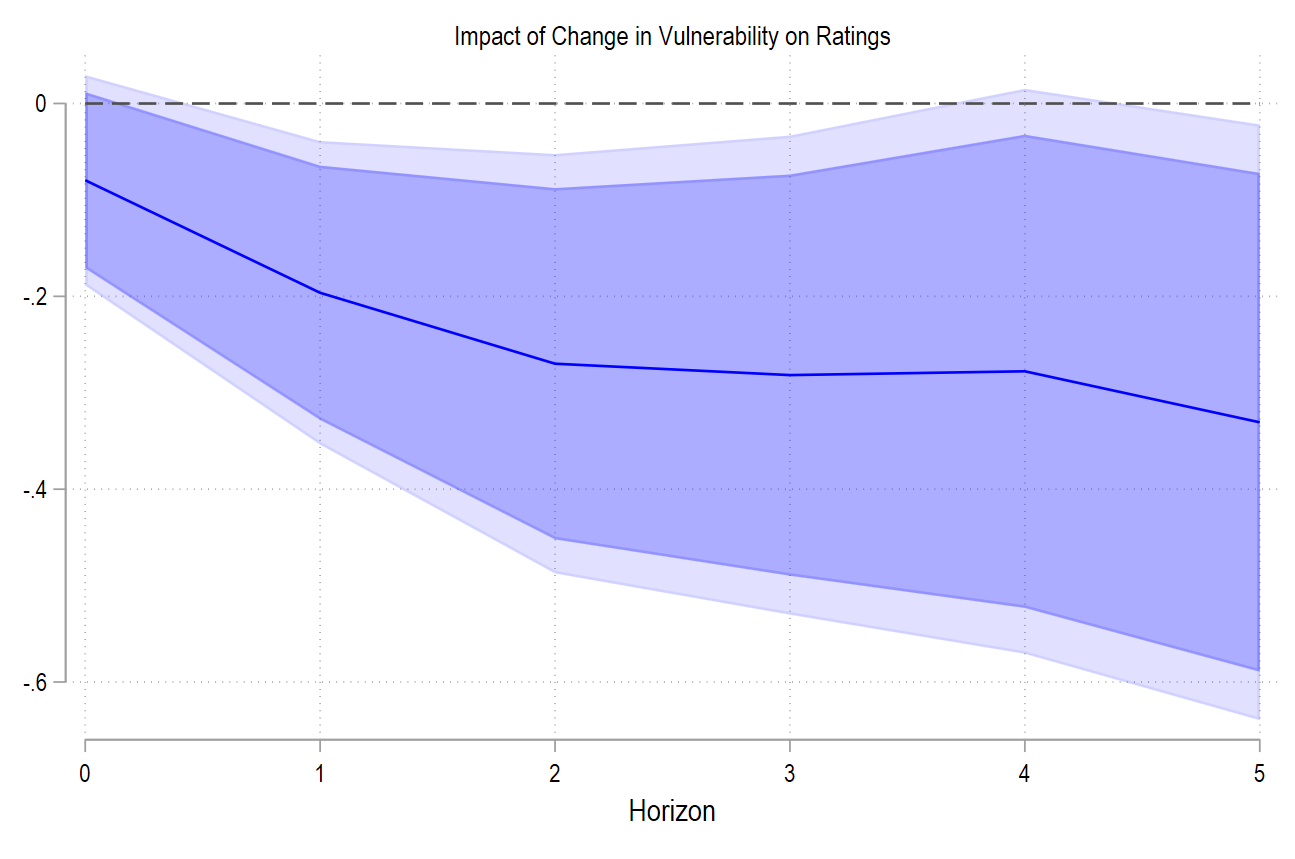
locproj sovrate, shock(Dvul100) ///
z h(5) yl(1) sl(3) ///
c(f(1/5).Dvul100 i.period) ///
fe cluster(imfcode) conf(90 95) ///
ttitle("Horizon") ///
title(`"Impact of Change in Vulnerability on Ratings"') ///
save irfname(sovrate_TZ) noisily stats grname(TZ2)
graph export sov_vul_jan25_TZ.png, as(png) width(4000) replace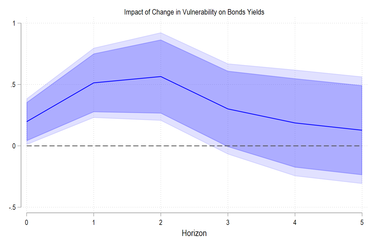
**# Teulings and Zubanov (Journal of Applied Econometrics 2014) show that including `forward' shocks variables resolve the misspecification problem
locproj bonds_tw, shock(D.pc1) ///
z h(4) yl(1) sl(5) ///
c(F(1/5).D.pc1 l(1).CAB l(1).cpi_tw l(1).GDebt l(1).GDeficit ///
l(1).banking l(1).currency l(1).debt i.period) ///
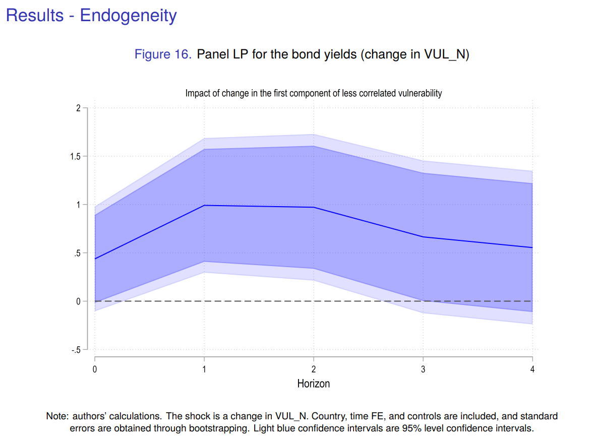
title("Impact of change in the first component of less correlated vulnerability") ///
ttitle("Horizon") ///
fe conf(90 95) noisily stats grname(TZ3)
graph export bond_pca_jan25_TZ.png, as(png) width(4000) replace
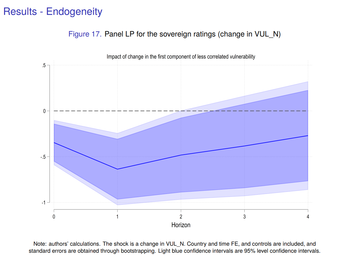
locproj sovrate, shock(D.pc1) ///
z h(4) yl(1) sl(5) ///
c(F(1/5).D.pc1 l(1).CAB l(1).cpi_tw l(1).GDebt l(1).GDeficit ///
l(1).banking l(1).currency l(1).debt i.period) ///
title("Impact of change in the first component of less correlated vulnerability") ///
ttitle("Horizon") ///
fe conf(90 95) noisily grname(TZ4)
graph export sovrate_pca_jan25_TZ.png, as(png) width(4000) replace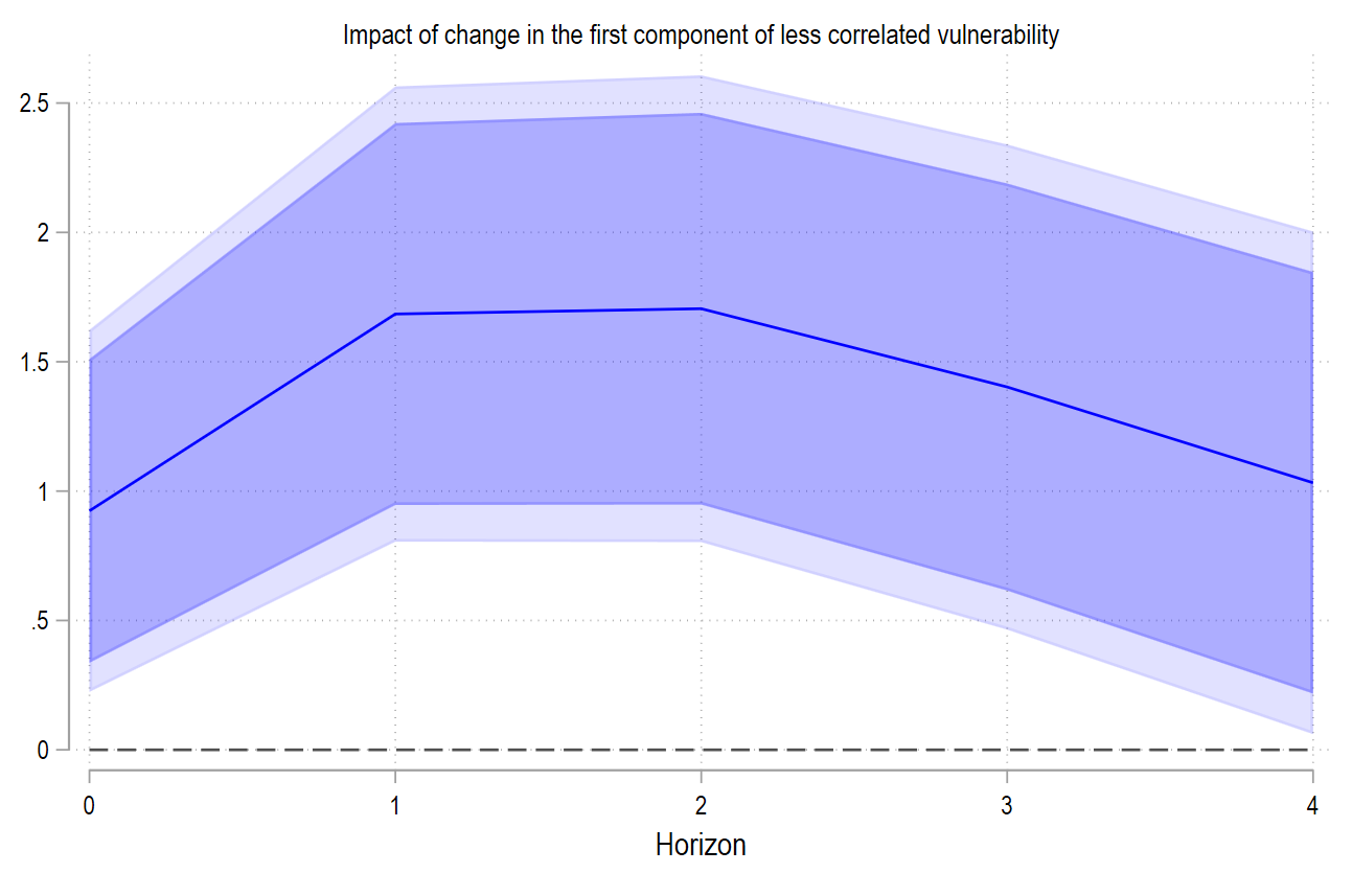
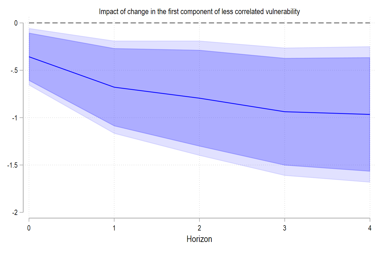
Our main results are confirmed when we control for future shocks, as recommended by Teulings and Zubanov, 2014.
References
Beirne, J., Park, D., Saadaoui, J., & Uddin, G. S. (2024). Impact of Climate Risk on Fiscal Space: Do Political Stability and Financial Development Matter? (No. 748). Asian Development Bank.
Kling, G., Volz, U., Murinde, V., & Ayas, S. (2021). The impact of climate vulnerability on firms’ cost of capital and access to finance. World Development, 137, 105131.
Teulings, C. N., & Zubanov, N. (2014). Is economic recovery a myth? Robust estimation of impulse responses. Journal of Applied Econometrics, 29(3), 497-514.