Sign and Narrative Restrictions in SVAR with Stata (Update August 2026) – Part II

In two earlier EconMacro posts, I introduced the VAR_NR package and discussed how to estimate structural vector autoregressions with long-run, short-run, sign, and narrative restrictions. The original post, Sign and Narrative Restrictions in SVAR with Stata, presented the toolbox. The April 2025 update then showed how to retrieve the series used to plot impulse-response functions, forecast-error variance decompositions, and historical decompositions.

In Part I of the August 2026 update, I explained how to recover the historical structural shocks from a point-identified Blanchard–Quah model. This second part addresses the more delicate case of sign and narrative restrictions.

The practical question is the following:

After estimating a sign- and narrative-restricted SVAR, how can we save the structural innovations as ordinary Stata variables and plot them against their historical dates?

The main complication is conceptual rather than computational. The Blanchard–Quah model in Part I produced one identified impact matrix and therefore one structural-shock history. Sign and narrative restrictions generally produce a set of admissible structural models. We must therefore preserve one complete accepted model—or carry all accepted models into the next stage—rather than combine pieces from different draws.

Structural shocks, impulse responses, and historical decompositions

Before turning to the code, it is useful to distinguish three related objects.

Object	What it measures	Index
Impulse-response function	The dynamic response of an endogenous variable to a hypothetical structural innovation	Horizon after the shock
Historical decomposition	The contribution of current and past structural shocks to the historical path of an endogenous variable	Calendar time and affected variable
Structural-shock series	The realized structural innovation in each period	Calendar time and shock

The structural shocks are not obtained by reading the historical-decomposition graph. Historical contributions already incorporate the propagation of the innovations through the complete VAR dynamics. Here we want the innovations before this dynamic propagation.

Step 1: Estimate the reduced-form VAR

The example uses quarterly observations for inflation, unemployment, and the federal funds rate. Let

y_t= \begin{pmatrix} \ln(\text{inflation}_t)\\ \ln(\text{unemployment}_t)\\ \ln(\text{federal funds rate}_t) \end{pmatrix}.

The reduced-form model is a VAR with two lags and a linear trend:

y_t=c+\Gamma t+A_1y_{t-1}+A_2y_{t-2}+u_t,

where

u_t= \begin{pmatrix} u_{\pi,t}\\u_{n,t}\\u_{i,t} \end{pmatrix}

contains the reduced-form forecast errors. The dataset runs from 1960Q1 to 2000Q4, giving 164 observations. Because the VAR contains two lags, the effective estimation sample begins in 1960Q3 and contains 162 residual observations.

The reduced-form residuals are observable after estimation, but they are not yet economically identified shocks. Their covariance matrix is

E(u_tu_t’)=\Sigma_u,

and its off-diagonal elements need not be zero.

Step 2: Define the structural representation

For an admissible structural model indexed by \(d\), write

u_t=B_d\varepsilon_t^{(d)}, \qquad E\!\left(\varepsilon_t^{(d)}\varepsilon_t^{(d)\prime}\right)=I.

The vector of structural innovations is

\varepsilon_t^{(d)}= \begin{pmatrix} \varepsilon_{S,t}^{(d)}\\ \varepsilon_{D,t}^{(d)}\\ \varepsilon_{MP,t}^{(d)} \end{pmatrix},

where the subscripts refer to supply, demand, and monetary policy shocks. The impact matrix is

B_d= \begin{pmatrix} b_{\pi S,d} & b_{\pi D,d} & b_{\pi MP,d}\\ b_{nS,d} & b_{nD,d} & b_{nMP,d}\\ b_{iS,d} & b_{iD,d} & b_{iMP,d} \end{pmatrix}.

Each column of \(B_d\) gives the contemporaneous responses of inflation, unemployment, and the federal funds rate to one structural shock. In the internal VAR_NR structure, this impact matrix is called inv_B0. Despite the name, it is the matrix that maps structural shocks into reduced-form innovations.

Step 3: Name the shocks and impose the sign restrictions

The ordering supplied to shock_name() determines the columns of the structural-shock matrix:

Column	Shock name	Saved Stata variable
1	Supply Shock	`shock_sr_supply`
2	Demand Shock	`shock_sr_demand`
3	Monetary Policy Shock	`shock_sr_monetary`

The identifying restrictions are imposed on impact because every shock_set() instruction uses periods 1 to 1.

Positive shock	Inflation	Unemployment	Federal funds rate
Supply shock	−	−	−
Demand shock	+	−	+
Monetary policy shock	−	+	+

The last row fixes the economic orientation of the monetary policy shock. A positive monetary policy innovation is a contractionary disturbance: the policy rate rises, unemployment rises, and inflation falls on impact. “Positive” is therefore a sign normalization; it does not mean that the shock is favorable for economic activity.

Because the restrictions apply only on impact, the responses are free to change sign at later horizons. A subsequent decline in the policy rate, for example, does not violate a restriction that requires the rate to rise only in the first response period.

Step 4: Add the narrative restriction

The narrative restriction requires the monetary policy shock to be positive in 1979Q4:

\varepsilon_{MP,1979Q4}^{(d)}>0.

Given the sign normalization above, this says that 1979Q4 must contain a contractionary monetary policy innovation. It is a restriction on the historical realization of the shock, not merely on the shape of an impulse response.

The condition does not require 1979Q4 to be the largest monetary policy shock in the sample. It does not require the shock to remain positive in nearby quarters, and it does not require monetary policy to be the dominant explanation of every macroeconomic movement around the Volcker disinflation. It requires only that the identified monetary policy innovation be positive at the selected date.

Step 5: Generate the accepted set

The command narr_sign_restrict() repeatedly draws candidate structural models. For each candidate, the routine:

draws reduced-form parameters;
draws an orthonormal rotation matrix \(Q_d\);
constructs the impact matrix;
checks the impact sign restrictions;
recovers the structural innovations needed to check the narrative restriction;
stores the complete model only when both sets of restrictions are satisfied.

For sign-restriction identification, the package constructs

\[ B_d=P_dQ_d’, \]

where \(P_d\) is the Cholesky factor associated with the draw-specific covariance matrix and \(Q_d\) is an accepted orthonormal rotation. The rotation preserves the covariance decomposition while changing the economic orientation of the shocks.

In this run, the algorithm attempted 86,451 candidate models. Of these, 2,016 satisfied the sign restrictions, and the routine continued until 1,000 models satisfied both the sign and narrative restrictions. These 1,000 complete accepted models are stored in the associative array SR.

Key point: SR is not a single estimated SVAR. It is a collection of admissible structural models. Each accepted element contains the objects needed to reproduce that model, including its parameter draw, covariance matrix, accepted rotation, and the reduced-form residual matrix used by the package.

Step 6: Summarize the accepted set with impulse responses

The command sr_analysis_funct("irf",SR,opts) computes the impulse responses for every accepted model. The plotted central line is the pointwise median across the 1,000 accepted IRFs, while the dashed lines form the central 68 percent interval requested through opts.pctg=68.

Impulse responses of inflation, unemployment, and the federal funds rate to a monetary policy shock under sign and narrative restrictions — **Figure 1.** Pointwise median impulse responses to a positive monetary policy shock, with central 68 percent bands across the accepted set. The restrictions require inflation to fall, unemployment to rise, and the federal funds rate to rise on impact. Later sign reversals are permitted.

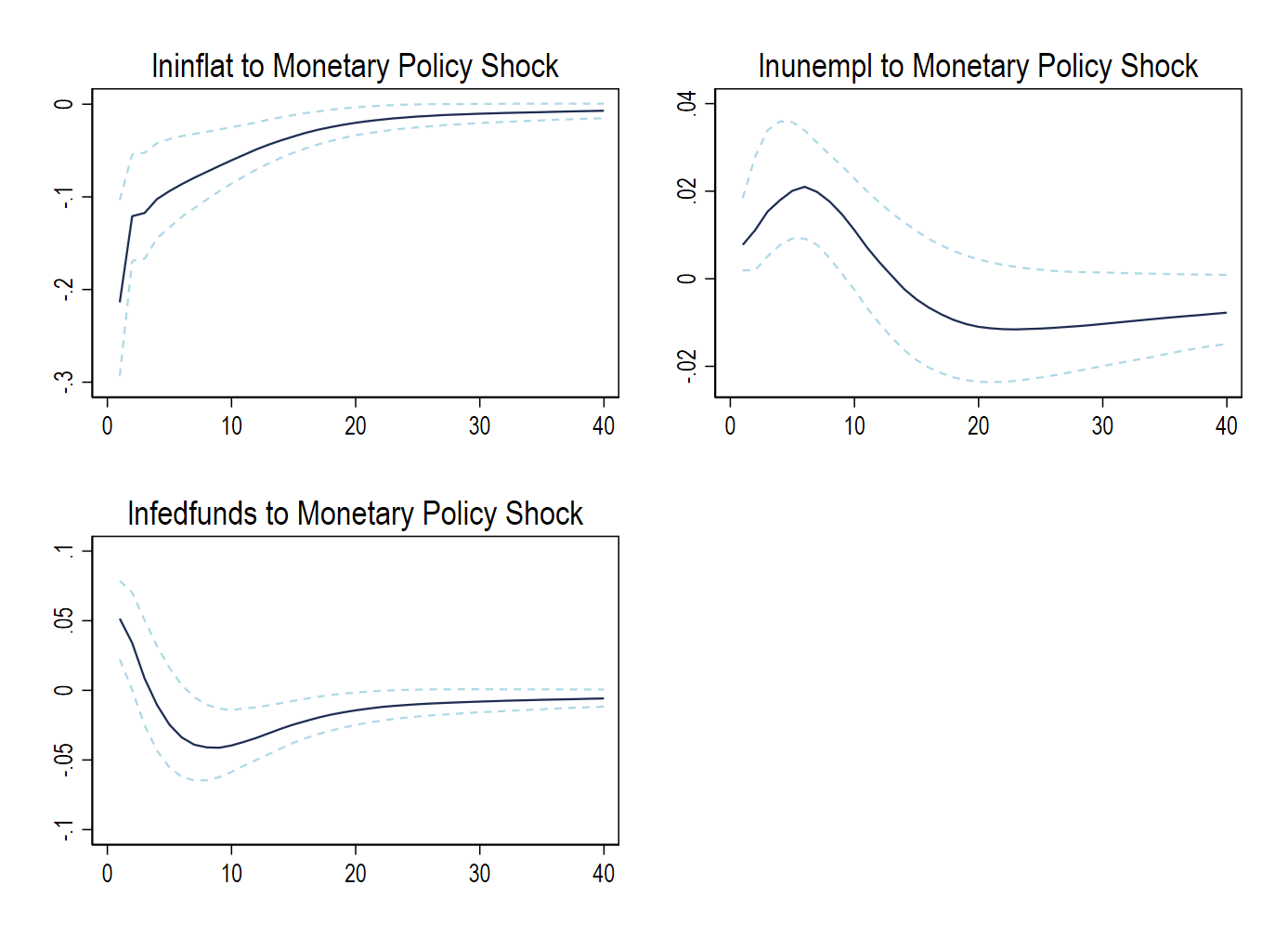
The figure illustrates the distinction between an impulse response and a historical shock. It asks what typically happens after a hypothetical one-standard-deviation monetary policy innovation. It does not tell us the size of the monetary policy innovation in a particular historical quarter.

Why we should not construct a pointwise median shock series

For every accepted model \(d\), there is a complete shock history:

\left\{\varepsilon_t^{(d)}\right\}_{t=1}^{T}.

It may appear natural to calculate the median shock separately at each date. But that operation can select the value from draw 17 in one quarter, draw 642 in the next quarter, and draw 91 in another quarter. The resulting sequence would generally not correspond to any single impact matrix, rotation matrix, or admissible structural model.

For the figures in this post, I therefore retain one complete accepted model: accepted draw 1. This is coherent because all dates use the same parameter draw, covariance matrix, rotation matrix, and impact matrix. It is also reproducible under the fixed seed, conditional on the same data, Stata environment, and package version.

Qualification: draw 1 is admissible, but it is not necessarily the most representative draw. The figures must therefore be described as the shocks from “accepted draw 1,” not as median structural shocks or as a uniquely identified shock history.

Step 7: Retrieve one complete accepted model

The helper Mata function receives the accepted-set object SR, the chosen draw number, and the option structure. It then retrieves

v_{\text{keep}}=SR[1].

Technically, the object must be declared as a struct var_struct scalar. The options copy must likewise be declared as a struct opt_struct scalar. These explicit declarations avoid Mata type-mismatch errors when assigning the accepted model and its option structure.

The command that sets the identification method to sr must remain inside Mata. If opts.ident="sr" is run as an ordinary Stata command, Stata interprets opts.ident as a command name and returns error r(199). Encapsulating the extraction in a Mata function prevents this mistake and makes the do-file easier to rerun.

Step 8: Reconstruct the impact matrix

The accepted model stores the covariance matrix and the accepted rotation \(Q_1\). The code clears the current impact matrix and calls identify(), which reconstructs

\[ B_1=P_1Q_1'. \]

The resulting \(3\times3\) matrix is stored internally as v_keep.inv_B0 and copied to the Stata matrix B_sr. The accepted rotation is copied to Q_sr. Keeping both matrices makes the retained contemporaneous identification transparent and inspectable.

Step 9: Recover the historical structural innovations

Starting from

u_t=B_1\varepsilon_t^{(1)},

the structural shocks are

\varepsilon_t^{(1)}=B_1^{-1}u_t.

The central Mata operation is

eps_keep = lusolve(v_keep.inv_B0,v_keep.U')'

This line is compact, so it is worth unpacking it carefully.

First, transpose the residual matrix

The stored residual matrix has dates in rows and variables in columns:

U= \begin{pmatrix} u_{\pi,1}&u_{n,1}&u_{i,1}\\ u_{\pi,2}&u_{n,2}&u_{i,2}\\ \vdots&\vdots&\vdots\\ u_{\pi,T}&u_{n,T}&u_{i,T} \end{pmatrix}.

Consequently, \(U’\) is a \(3\times T\) matrix in which each column contains the three reduced-form innovations for one quarter.

Second, solve the structural system

lusolve(B,U') solves

\[ BX=U’ \]

for \(X\). Therefore,

X=B^{-1}U’= \begin{pmatrix} \varepsilon_{S,1}&\cdots&\varepsilon_{S,T}\\ \varepsilon_{D,1}&\cdots&\varepsilon_{D,T}\\ \varepsilon_{MP,1}&\cdots&\varepsilon_{MP,T} \end{pmatrix}.

Using lusolve() is preferable to explicitly forming a matrix inverse. It directly solves the linear system and follows the same transformation used internally by the package when it checks narrative restrictions and constructs historical decompositions.

Third, transpose the result back

The final apostrophe returns a \(T\times3\) matrix:

eps\_keep= \begin{pmatrix} \varepsilon_{S,1}&\varepsilon_{D,1}&\varepsilon_{MP,1}\\ \varepsilon_{S,2}&\varepsilon_{D,2}&\varepsilon_{MP,2}\\ \vdots&\vdots&\vdots\\ \varepsilon_{S,T}&\varepsilon_{D,T}&\varepsilon_{MP,T} \end{pmatrix}.

Rows are now dates and columns are structural shocks, which is precisely the organization required to transfer the matrix into Stata variables.

Step 10: Align the shocks with calendar time

The original dataset has 164 quarterly observations, but the two-lag VAR produces only 162 residual observations. The code calculates

\text{first observation}=164-162+1=3.

The first two quarters—1960Q1 and 1960Q2—remain missing because they are needed to construct the lags. The first recovered shock is assigned to 1960Q3, which is the beginning of the effective VAR sample.

Stata observation	Quarter	Structural-shock value
1	1960Q1	Missing
2	1960Q2	Missing
3	1960Q3	First recovered innovation
⋮	⋮	⋮
164	2000Q4	Final recovered innovation

Step 11: Transfer the shocks to Stata and validate them

Before entering Mata, the code creates three empty Stata variables. The st_store() command then transfers the three columns of eps_keep into shock_sr_supply, shock_sr_demand, and shock_sr_monetary.

The most important numerical diagnostic verifies that the recovered shocks reconstruct the reduced-form innovations:

U’=B_1\varepsilon^{(1)\prime}.

The code computes the maximum absolute discrepancy across every variable and every date:

\max_{i,t}\left|U’_{i,t}-\left(B_1\varepsilon^{(1)\prime}\right)_{i,t}\right|.

This number should be extremely close to zero, typically at floating-point precision. The check confirms that the matrix orientation, column ordering, and extraction formula are correct. It does not test whether the identifying assumptions are economically compelling; that remains a substantive modeling judgment.

Supply, demand, and monetary policy structural shocks from accepted draw 1 under sign and narrative restrictions — **Figure 2.** Historical structural innovations from one complete accepted model, draw 1. The vertical line marks 1979Q4. These series are structural shocks indexed by calendar time; they are not impulse responses or historical contributions.

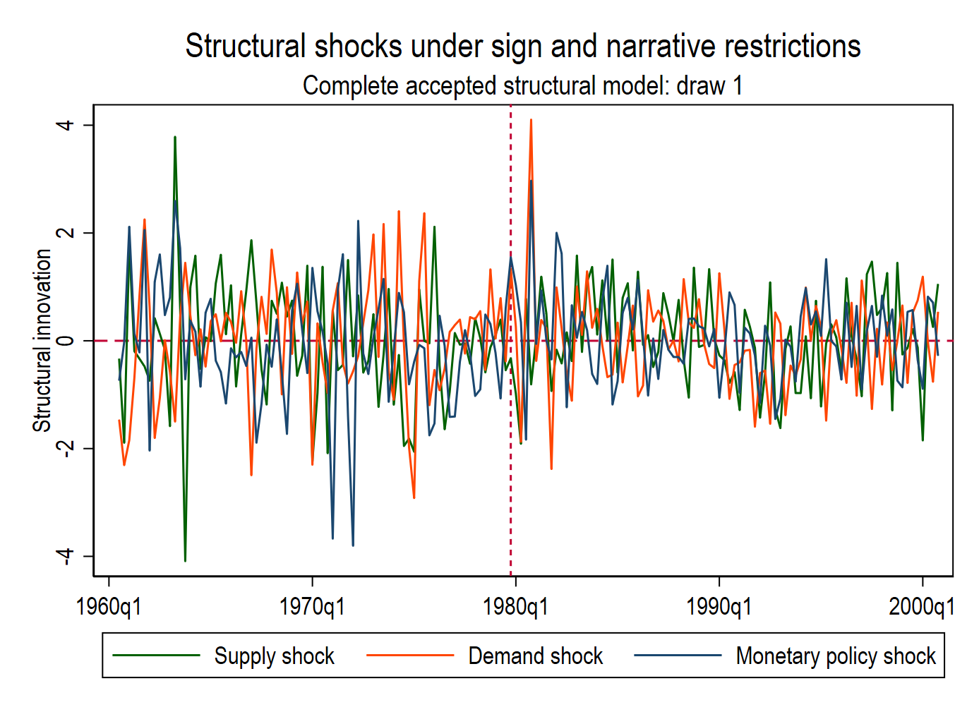
How to read the three-shock figure

Each line reports the standardized structural innovation associated with one shock in accepted draw 1. A value of 2 means a relatively large positive innovation under that draw’s normalization. It does not mean that inflation, unemployment, or the federal funds rate moved by two percentage points.

The contemporaneous reduced-form innovations are obtained by multiplying the structural-shock vector by the impact matrix:

\begin{pmatrix} u_{\pi,t}\\u_{n,t}\\u_{i,t} \end{pmatrix} = B_1 \begin{pmatrix} \varepsilon_{S,t}^{(1)}\\ \varepsilon_{D,t}^{(1)}\\ \varepsilon_{MP,t}^{(1)} \end{pmatrix}.

The observed macroeconomic variables also depend on their lagged histories, the deterministic terms, and the propagation of past shocks. The figure is therefore a graph of innovations, not a graph of observed inflation, unemployment, or interest rates.

Step 12: Verify the narrative restriction directly

The code does not merely rely on the package’s acceptance decision. After storing the monetary policy shock as a Stata variable, it performs an explicit check:

\varepsilon_{MP,1979Q4}^{(1)}>0.

The assert command makes this an executable diagnostic. If the recovered shock were zero or negative in 1979Q4, Stata would stop with an error.

Monetary policy structural shock from accepted draw 1 with the 1979Q4 narrative restriction marked — **Figure 3.** Monetary policy structural innovation from accepted draw 1. The vertical line marks 1979Q4, when the narrative restriction requires the shock to be positive.

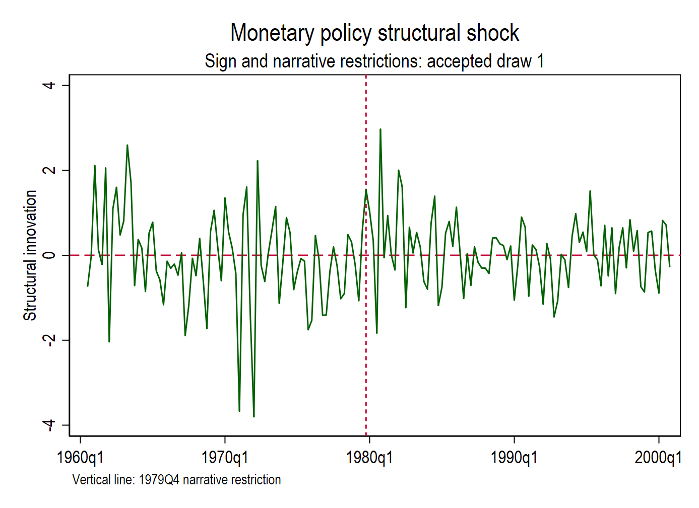
The monetary policy innovation is positive at the vertical line, as required. A larger positive realization appears shortly afterward. This does not contradict the narrative restriction, because the restriction fixes only the sign in 1979Q4; it does not require that date to contain the largest tightening shock in the sample.

Negative realizations of the series correspond to expansionary monetary policy innovations under the adopted sign normalization. Again, this classification refers to the identified innovation, not directly to the observed quarterly change in the federal funds rate.

One accepted draw or the full accepted set?

The appropriate treatment depends on the purpose of the exercise.

Purpose	Recommended treatment
Illustrate how to recover and save a coherent shock history	Retain one explicitly documented accepted draw
Inspect candidate historical events	Use one or several accepted draws and report sensitivity
Estimate a second-stage regression or local projection	Repeat the second stage across accepted draws and summarize the resulting distribution
Summarize impulse responses	Use the median and bands produced across the accepted set
Create a “median shock history” date by date	Avoid treating it as a single accepted structural model

For a published second-stage exercise, carrying identification uncertainty through the accepted draws is preferable. The draw-1 series in this post is primarily a transparent and internally coherent illustration of the extraction procedure.

Conclusion

Recovering structural shocks under sign and narrative restrictions requires one additional decision that does not arise in a point-identified model: we must decide how to handle the set of accepted structural models.

The procedure used here is:

\boxed{ \begin{aligned} \text{Estimate the reduced-form VAR} &\longrightarrow (A,\Sigma,U),\\ \text{draw parameters and rotations} &\longrightarrow (A_d,\Sigma_d,Q_d),\\ \text{impose sign restrictions} &\longrightarrow \text{sign-admissible models},\\ \text{impose }\varepsilon_{MP,1979Q4}^{(d)}>0 &\longrightarrow SR,\\ \text{retain one complete accepted draw} &\longrightarrow (B_1,Q_1),\\ \varepsilon_t^{(1)}=B_1^{-1}u_t &\longrightarrow \text{saved Stata shock series}. \end{aligned} }

The essential Mata calculation remains simple:

eps_keep = lusolve(v_keep.inv_B0,v_keep.U')'

The care is needed around that line: use a complete accepted draw, preserve the shock ordering, align the residual sample with the original dates, and verify both the algebraic reconstruction and the narrative restriction. Once those steps are completed, the supply, demand, and monetary policy innovations are ordinary Stata variables that can be plotted, exported, and used in subsequent analysis.

Complete Stata code

The following code reproduces the accepted-set estimation, calculates and exports the monetary policy IRFs, retrieves the structural innovations from accepted draw 1, validates them, plots the three shocks, plots the monetary policy shock separately, and saves a clean shock dataset.

////////////////////////////////////////////////////////////////

**# /* Narrative Sign Restrictions */

/*
Keep in mind that code for these functions is adapted
from Ambrogio Cesa-Bianchi's VAR Toolbox.

The code follows the notation in Kilian and Lütkepohl,
Structural Vector Autoregressive Analysis (2016),
including the IRF, FEVD, and HD calculations.
*/

clear *
use data_narrsignrestrict, clear
tsset date

// -----------------------------------------------------------------------------
// Estimate the reduced-form VAR
// -----------------------------------------------------------------------------

var lninflat lnunempl lnfedfunds, ///
    lags(1/2)                     ///
    exog(trend)

var_nr sr,                        ///
    varname("v")                  ///
    opt("opts")                   ///
    lintrend(trend)

var_nr_options_display, optname("opts") all

// -----------------------------------------------------------------------------
// Narrative date and accepted draw to retain
// -----------------------------------------------------------------------------

local Volcker_disinfl_pf = yq(1979,4)

// Retain one complete accepted structural model.
// With the fixed seed, draw 1 is reproducible.
local keep_draw = 1

// -----------------------------------------------------------------------------
// Create variables that will receive the structural innovations
// -----------------------------------------------------------------------------

capture drop shock_sr_supply
capture drop shock_sr_demand
capture drop shock_sr_monetary

generate double shock_sr_supply   = .
generate double shock_sr_demand   = .
generate double shock_sr_monetary = .

// -----------------------------------------------------------------------------
// Remove the helper Mata function if this do-file has already been run
// -----------------------------------------------------------------------------

capture mata: mata drop _var_nr_save_sr_shocks()

mata

// -----------------------------------------------------------------------------
// Helper function: extract the shocks from one complete accepted draw
// -----------------------------------------------------------------------------

void function _var_nr_save_sr_shocks(
    transmorphic scalar SR,
    real scalar keep_draw,
    struct opt_struct scalar opts)
{
    struct var_struct scalar v_keep
    struct opt_struct scalar opts_keep

    real matrix eps_keep
    real colvector obs_keep

    real scalar first_obs_keep
    real scalar reconstruction_error

    // Check that the requested accepted draw exists
    if (keep_draw<1 | keep_draw>asarray_elements(SR)) {
        _error("keep_draw is outside the range of accepted draws")
    }

    // Retrieve one complete accepted structural model
    v_keep = asarray(SR,keep_draw)

    // Make a correctly typed copy of the option structure
    opts_keep = opts
    opts_keep.ident = "sr"

    // Reconstruct the contemporaneous structural impact matrix
    //
    // Under sign restrictions:
    //
    //     B = P Q'
    //
    // where P is based on the Cholesky factor of sigma and Q is the
    // accepted orthonormal rotation matrix.

    v_keep.inv_B0 = J(0,0,.)
    identify(v_keep,opts_keep)

    // Recover the structural innovations:
    //
    //     U' = B epsilon'
    //
    // and therefore:
    //
    //     epsilon' = B^(-1) U'
    //
    // The final transpose gives dates x structural shocks.

    eps_keep = lusolve(v_keep.inv_B0,v_keep.U')'

    // Match the rows of the structural-shock matrix to Stata observations
    //
    // In this application:
    //
    //     nobs           = 164
    //     rows(eps_keep) = 162
    //
    // Therefore, the shocks begin at observation 3 because the VAR
    // uses two lags.

    first_obs_keep = v_keep.nobs - rows(eps_keep) + 1
    obs_keep = (first_obs_keep::v_keep.nobs)

    // Verify the time-series alignment
    if (rows(eps_keep)!=rows(obs_keep)) {
        _error("Structural-shock/sample alignment failed")
    }

    // Transfer the structural innovations to the Stata dataset
    //
    // Column ordering follows shock_name():
    //
    //     column 1 = Supply Shock
    //     column 2 = Demand Shock
    //     column 3 = Monetary Policy Shock

    st_store(
        obs_keep,
        (
            "shock_sr_supply",
            "shock_sr_demand",
            "shock_sr_monetary"
        ),
        eps_keep
    )

    // Store the identifying matrices in Stata
    st_matrix("B_sr",v_keep.inv_B0)
    st_matrix("Q_sr",v_keep.Q)

    // Store the accepted-draw number
    st_numscalar("kept_sr_draw",keep_draw)

    // Verify that B times the recovered shocks reconstructs U
    reconstruction_error = max(
        abs(
            vec(
                v_keep.U' -
                v_keep.inv_B0*eps_keep'
            )
        )
    )

    st_numscalar(
        "sr_reconstruction_error",
        reconstruction_error
    )
}

// -----------------------------------------------------------------------------
// Create narrative restrictions
// -----------------------------------------------------------------------------

ns = nr_create(v)

nr_set(
    yq(1979,4),
    yq(1979,4),
    "+",
    "Monetary Policy Shock",
    "",
    ns
)

// -----------------------------------------------------------------------------
// Create sign restrictions
// -----------------------------------------------------------------------------

s = shock_create(v)

shock_name(
    (
        "Supply Shock",
        "Demand Shock",
        "Monetary Policy Shock"
    ),
    s
)

// Supply shock

shock_set(1,1,"-","Supply Shock","lninflat",s)
shock_set(1,1,"-","Supply Shock","lnunempl",s)
shock_set(1,1,"-","Supply Shock","lnfedfunds",s)

// Demand shock

shock_set(1,1,"+","Demand Shock","lninflat",s)
shock_set(1,1,"-","Demand Shock","lnunempl",s)
shock_set(1,1,"+","Demand Shock","lnfedfunds",s)

// Monetary policy shock

shock_set(1,1,"-","Monetary Policy Shock","lninflat",s)
shock_set(1,1,"+","Monetary Policy Shock","lnunempl",s)
shock_set(1,1,"+","Monetary Policy Shock","lnfedfunds",s)

// -----------------------------------------------------------------------------
// Set options
// -----------------------------------------------------------------------------

opts = opt_set()

opts.ndraws     = 1000
opts.updt       = "yes"
opts.updt_frqcy = 1000
opts.pctg       = 68
opts.save_fmt   = "png"

// Plot the responses of all endogenous variables to the monetary policy shock
opts.shck_plt = "Monetary Policy Shock"

opt_display(opts)

// -----------------------------------------------------------------------------
// Estimate the sign- and narrative-restricted model
// -----------------------------------------------------------------------------

stata("set seed 123456")

SR = narr_sign_restrict(v,s,opts,ns)

// -----------------------------------------------------------------------------
// Recover the structural innovations from accepted draw 1
// -----------------------------------------------------------------------------

_var_nr_save_sr_shocks(
    SR,
    `keep_draw',
    opts
)

// -----------------------------------------------------------------------------
// Calculate and plot the IRFs
// -----------------------------------------------------------------------------

IRF_set = sr_analysis_funct(
    "irf",
    SR,
    opts
)

irf_plot(
    asarray(IRF_set,"median"),
    asarray(IRF_set,"bands"),
    v,
    opts
)

// Because opts.save_fmt="png", irf_plot() saves:
// IRF_Monetary_Policy_Shock.png

end

// -----------------------------------------------------------------------------
// Label the recovered structural shocks
// -----------------------------------------------------------------------------

label variable shock_sr_supply ///
    "Supply structural shock: accepted draw `keep_draw'"

label variable shock_sr_demand ///
    "Demand structural shock: accepted draw `keep_draw'"

label variable shock_sr_monetary ///
    "Monetary policy structural shock: accepted draw `keep_draw'"

// -----------------------------------------------------------------------------
// Label and inspect the identifying matrices
// -----------------------------------------------------------------------------

matrix rownames B_sr = ///
    lninflat         ///
    lnunempl         ///
    lnfedfunds

matrix colnames B_sr = ///
    supply           ///
    demand           ///
    monetary

matrix rownames Q_sr = ///
    q1               ///
    q2               ///
    q3

matrix colnames Q_sr = ///
    supply           ///
    demand           ///
    monetary

matrix list B_sr
matrix list Q_sr

// -----------------------------------------------------------------------------
// Diagnostics
// -----------------------------------------------------------------------------

display "Accepted draw retained = " ///
    %9.0f scalar(kept_sr_draw)

display "Maximum reconstruction error = " ///
    %12.4e scalar(sr_reconstruction_error)

summarize ///
    shock_sr_supply ///
    shock_sr_demand ///
    shock_sr_monetary

correlate ///
    shock_sr_supply ///
    shock_sr_demand ///
    shock_sr_monetary

// Verify the narrative restriction
list date shock_sr_monetary ///
    if date==`Volcker_disinfl_pf', ///
    noobs

assert shock_sr_monetary>0 ///
    if date==`Volcker_disinfl_pf'

// -----------------------------------------------------------------------------
// Plot all three structural shocks
// -----------------------------------------------------------------------------

set scheme s1color

tsline ///
    shock_sr_supply ///
    shock_sr_demand ///
    shock_sr_monetary, ///
    yline(0, lpattern(dash)) ///
    xline(`Volcker_disinfl_pf', lpattern(shortdash)) ///
    title("Structural shocks under sign and narrative restrictions") ///
    subtitle("Complete accepted structural model: draw `keep_draw'") ///
    xtitle("") ///
    ytitle("Structural innovation") ///
    legend( ///
        order( ///
            1 "Supply shock" ///
            2 "Demand shock" ///
            3 "Monetary policy shock" ///
        ) ///
        rows(1) ///
    ) ///
    name(sr_all_structural_shocks, replace)

graph save ///
    "sr_all_structural_shocks.gph", ///
    replace

graph export ///
    "sr_all_structural_shocks.png", ///
    width(2400) ///
    replace

// -----------------------------------------------------------------------------
// Plot the monetary policy shock separately
// -----------------------------------------------------------------------------

tsline shock_sr_monetary, ///
    yline(0, lpattern(dash)) ///
    xline(`Volcker_disinfl_pf', lpattern(shortdash)) ///
    title("Monetary policy structural shock") ///
    subtitle("Sign and narrative restrictions: accepted draw `keep_draw'") ///
    xtitle("") ///
    ytitle("Structural innovation") ///
    legend(off) ///
    note("Vertical line: 1979Q4 narrative restriction") ///
    name(sr_monetary_structural_shock, replace)

graph save ///
    "sr_monetary_structural_shock.gph", ///
    replace

graph export ///
    "sr_monetary_structural_shock.png", ///
    width(2400) ///
    replace

// -----------------------------------------------------------------------------
// Save a clean structural-shock dataset
// -----------------------------------------------------------------------------

preserve

keep ///
    date ///
    shock_sr_supply ///
    shock_sr_demand ///
    shock_sr_monetary

drop if missing(shock_sr_monetary)

compress

save ///
    "sr_structural_shocks_draw`keep_draw'.dta", ///
    replace

restore

Practical point: run the entire Mata section—from mata through end—as one block. Running only part of it from the Do-file Editor can produce an “end statement missing” error or cause Mata assignments to be interpreted as Stata commands.