Sign and Narrative Restrictions in SVAR with Stata

Today I will present you VAR_NR, a Stata module to estimate set identified Structural VAR. This toolbox has been provided by Abigail Kuchek (abigail.kuchek@dal.frb.org), Jonah Danziger (jonah.danziger@dal.frb.org) and Christoffer Koch.

On EconPapers, you will find the abstract describing the routine:

The toolbox var_nr allows for the estimation of set identified SVARS in Stata using sign and narrative restrictions. The suite can produce impulse responses functions, forecast error variance decompositions, and historical decompositions. These postestimation commands can also be used in conjunction with standard point identified SVARs with short- or long-run restrictions.

First, you have to install the package from SSC:

ssc install var_nr

Then, you have to consult the documentation, which is very extensive:

help var_nr

As mentioned in the help, keep in mind that ident specifies the method for identifying the VAR. This option will accept one of three strings: “oir“, “bq“, or “sr“. “oir” specifies zero short-run restrictions; “bq” specifies zero long-run restrictions (Blanchard and Quah, I presume); and “sr” specifies [narrative] sign restrictions.

Besides, it is also mentioned that the code for several Mata functions are based on the following sources from Ambrogio Cesa-Bianchi’s VAR Toolbox, and follows Kilian and Lutkepohl’s notation in Structural Vector Autoregressive Analysis (2016). Also for IRF, HD and FEDV.

In the following, I reproduce their examples and I show how to change some options (in bold, type help var_nr_options for more details), we start with zero-long run restrictions:

**# /* Long-run Zero Restrictions */

clear *
use data_longrun
tsset date

// estimate var
var GDPGrowth Unemployment, lags(1/4)
var_nr bq, var("VAR") opt("opts")
var_nr_options_display , optname("opts") all

// Change options

var_nr_options , optname("opts") savefmt("png") pctg(68)
var_nr_options_display , optname("opts") all

mata
// only plot GDP growth
opts.shck_plt = "GDPGrowth"

// compute IRF, bands, plot
IRF = irf_funct(VAR,opts)
IRFB = irf_bands_funct(VAR,opts)
irf_plot(IRF,IRFB,VAR,opts)

// compute FEVD, bands, plot
FEVD = fevd_funct(VAR,opts)
FEVDB = fevd_bands_funct(VAR,opts)
fevd_plot(FEVD,FEVDB,VAR,opts)

// compute HD, plot
HD = hd_funct(VAR,opts)
hd_plot(HD,VAR,opts)
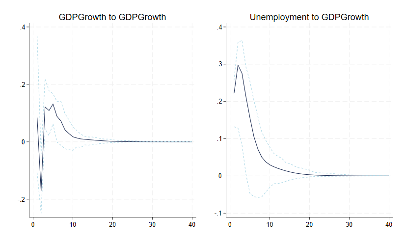
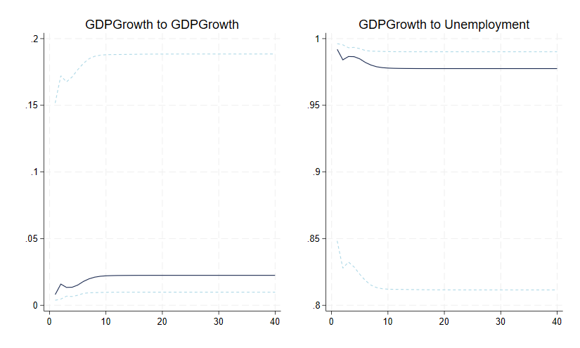
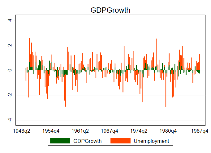
end

The code has to be run entirely, it produces the following graphs for IRF, FEVD and HD:

Impulse Response Function

Forecast Error Variance Decomposition

Historical Decomposition

Now, we have the Narrative signs restrictions:

**# /* Narrative Sign Restrictions */

/*
Keep in mind that Code for this function is adapted 
from Ambrogio Cesa-Bianchi's VAR Toolbox.  
Code follows Kilian and Lutkepohl's notation in Structural 
Vector Autoregressive Analysis (2016). Also for IRF, HD and 
FEDV.
*/

clear *
use data_narrsignrestrict
tsset date

// estimate var
var lninflat lnunempl lnfedfunds, lags(1/2) exog(trend)
var_nr sr, varname("v") opt("opts") lintrend(trend)
var_nr_options_display , optname("opts") all

// narrative restriction: positive Oct 79 (q4 '79)
loc Volcker_disinfl_pf = yq(1979,4)

mata
ns = nr_create(v)
nr_set(yq(1979,4),yq(1979,4),"+","Monetary Policy Shock","",ns)

// load matrices into associative array to prep for calculations
s = shock_create(v)
shock_name(("Supply Shock","Demand Shock","Monetary Policy Shock"),s)

shock_set(1,1,"-","Supply Shock","lninflat",s)
shock_set(1,1,"-","Supply Shock","lnunempl",s)
shock_set(1,1,"-","Supply Shock","lnfedfunds",s)

shock_set(1,1,"+","Demand Shock","lninflat",s)
shock_set(1,1,"-","Demand Shock","lnunempl",s)
shock_set(1,1,"+","Demand Shock","lnfedfunds",s)

shock_set(1,1,"-","Monetary Policy Shock","lninflat",s)
shock_set(1,1,"+","Monetary Policy Shock","lnunempl",s)
shock_set(1,1,"+","Monetary Policy Shock","lnfedfunds",s)

// set options
opts = opt_set()
opts.ndraws = 1000
opts.updt = "yes"
opts.updt_frqcy = 1000
*Additional options
opts.save_fmt="png"
opts.pctg=68
opt_display(opts)

// run narrative sign restrictions routine
stata("set seed 123456")
SR = narr_sign_restrict(v,s,opts,ns)

// IRF, FEVD, HD calculations
IRF_set = sr_analysis_funct("irf",SR,opts)
FEVD_set = sr_analysis_funct("fevd",SR,opts)
HD_set = sr_analysis_funct("hd",SR,opts)

// plot and save
irf_plot(asarray(IRF_set,"median"),asarray(IRF_set,"bands"),v,opts)
fevd_plot(asarray(FEVD_set,"median"),asarray(FEVD_set,"bands"),v,opts)
hd_plot(asarray(HD_set,"median"),v,opts)
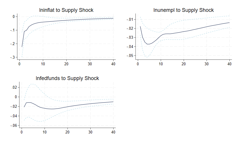
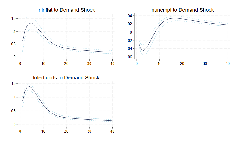
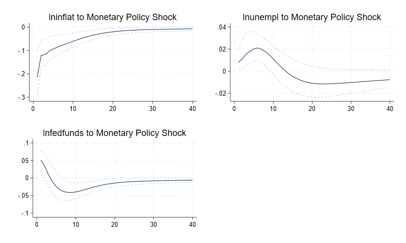
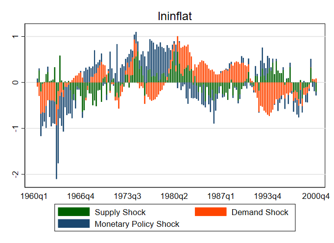
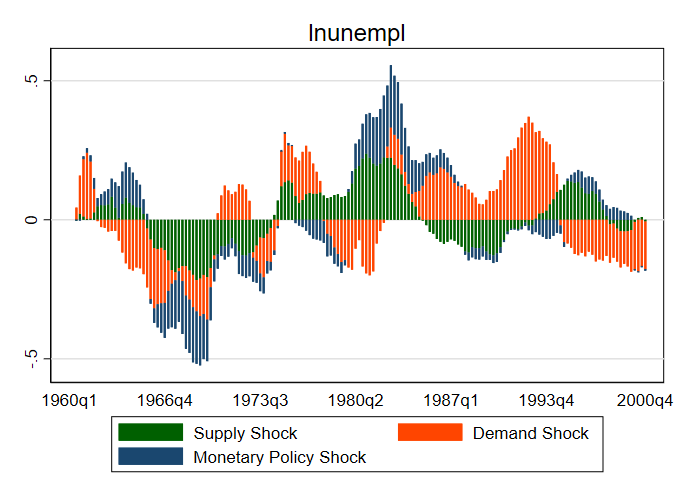
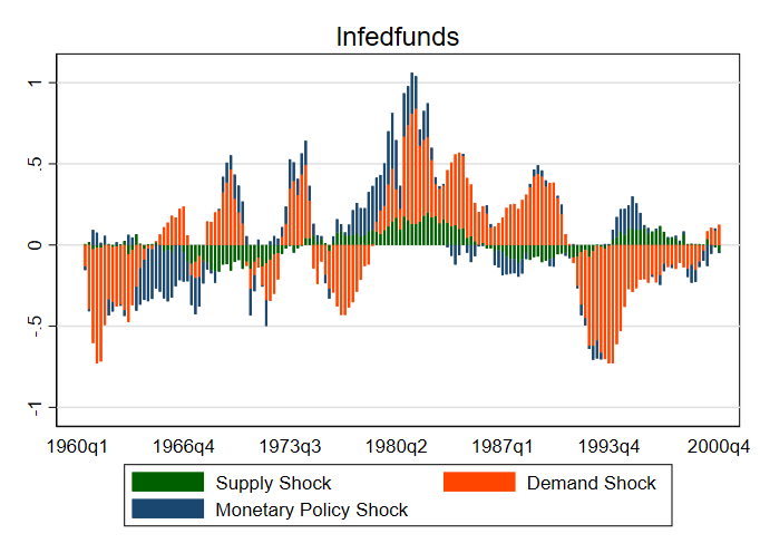
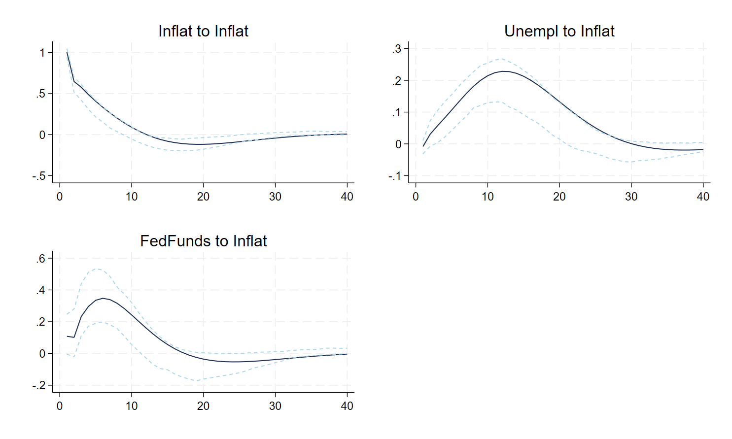
end

The code has to be run entirely, it produces the following graphs for IRF, FEVD and HD:

Impulse Response Function

Forecast Error Variance Decomposition

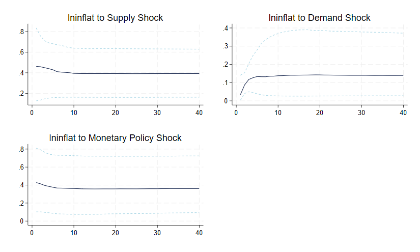
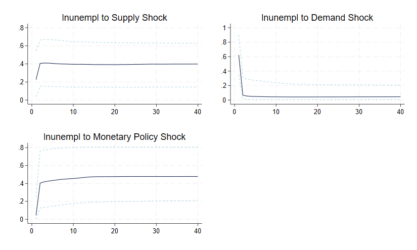
Historical Decomposition

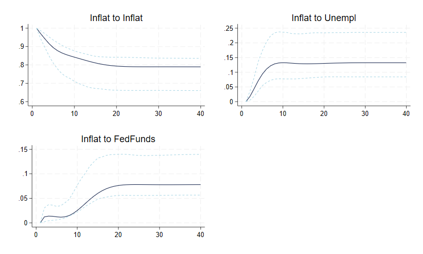
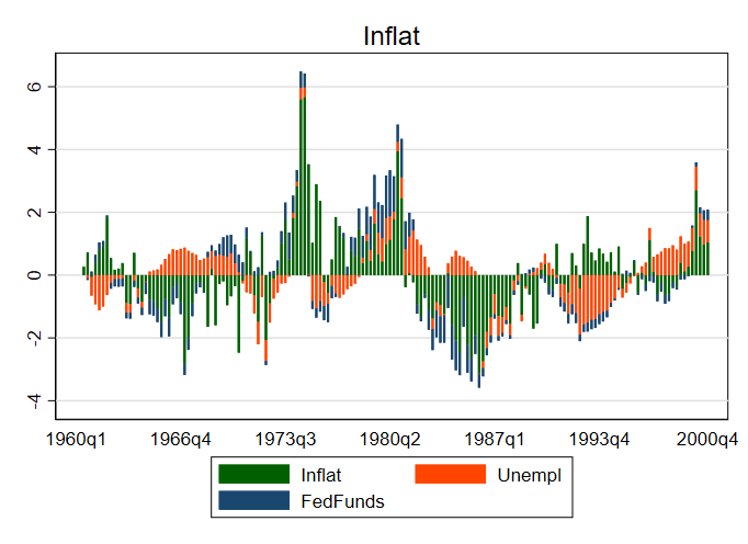
Now, we will demonstrate the Short-run Zero Restrictions. Do not forget to erase (or better rename the PNG files with ‘LR’ suffix) the graph that you had with the Long-run Zero Restrictions:

**# /* Short-run Zero Restrictions */

clear *
use data_shortrun
tsset date

// estimate var
var Inflat Unempl FedFunds, lags(1/2) exog(trend trendsq)
var_nr oir, varname("VAR") optname("A") lintr(trend) quadtr(trendsq)
var_nr_options_display , optname("A") all

mata
// only plot Inflation
A.shck_plt = "Inflat"
*Additional options
A.save_fmt="png"
A.pctg=68
opt_display(A)

// IRF
IRF = irf_funct(VAR,A)
IRFB = irf_bands_funct(VAR,A)

// FEVD
FEVD = fevd_funct(VAR,A)
FEVDB = fevd_bands_funct(VAR,A)

// HD
HD = hd_funct(VAR,A)

// plot all of the above
irf_plot(IRF,IRFB,VAR,A)
fevd_plot(FEVD,FEVDB,VAR,A)
hd_plot(HD,VAR,A)
end

Impulse Response Function

Forecast Error Variance Decomposition

Historical Decomposition

As we have seen in this blog, this toolbox allows estimating sign and narrative restrictions in Stata. The files for replicating this blog are available on my GitHub.