A Teulings-Zubanov-Style Correction for LP-IV Models with Stata

This blog was inspired by a discussion with Davide Romelli at the SILVAPLANA POLITICAL ECONOMY 2026 workshop. Davide suggested that I include future values of the shock in my local-projection instrumental-variable specification à la Teulings and Zubanov (2014).

The modification looks simple at first glance. However, the Teulings-Zubanov-qstyle correction is used in a standard local projection setup, not in a local-projection instrumental-variable specification. In order to adapt Teulings-Zubanov correction in Stata, I retain the contemporaneous geopolitical turning point as the excluded instrument and add its first two future realizations as controls:

F(1/2).d2pri

Econometrically, however, the modification is important. It changes the source of identifying variation and therefore the dynamic causal object estimated by the LP-IV.

The central idea is:

Keep the contemporaneous external instrument as the excluded instrument, but partial out its future realizations.

This procedure extends the intuition of Teulings and Zubanov to an LP-IV setting. It is not a literal replication of their estimator, because they control for future realizations of an event or treatment, whereas I control for future realizations of an external instrument. The procedure is therefore best described as a Teulings-Zubanov-style lead augmentation for LP-IV.

This blog also extends an earlier EconMacro post in which I used forward shocks in standard local projections estimated with locproj. I recommand reading the following blogs before diving into this one:

• Adding Forward Shocks to Solve Misspecification in Local Projections with LOCPROJ.
• Thou Shalt Lag-Augment, Not “Stationarize” when Using Local Projections.
• Can Local Projections Have Short-Run Restrictions?
• Geopolitical Turning Points and Macroeconomic Volatility: Relevance, Anticipation, and Exclusion (Honey, I think I found an instrument)

The dataset come the following research article:

Saadaoui, J. (2026). Geopolitical turning points and macroeconomic volatility: A bilateral identification strategy. Journal of Comparative Economics. 10.1016/j.jce.2026.03.010

1. The baseline LP-IV model

Consider the horizon-specific local projection:

$$y_{t+h} = \alpha_h +\beta_h x_t +\Gamma_h’W_t +u_{t+h}, \qquad h=0,\ldots,H,$$

where:

• $y_{t+h}$ is the outcome at horizon $h$;
• $x_t$ is the endogenous impulse variable;
• $W_t$ contains lags and other controls;
• $z_t$​ is an external instrument for $x_t$​;
• $\beta_h$ is the horizon-specific response.

The corresponding first stage is:

$$x_t = \pi_h z_t +\Lambda_h’W_t +v_{t,h}.$$

The LP-IV uses variation in $x_t$​ generated by the external instrument $z_t$​. This is the direct, one-step external-instrument implementation of local projections.

At positive horizons, however, the outcome may also be affected by geopolitical innovations occurring after $t$:

$$y_{t+h} = \beta_h x_t +\sum_{j=1}^{h}\theta_{j,h}x_{t+j} +\varepsilon_{t+h}.$$

When that is the case, the baseline LP-IV can combine the effect of the contemporaneous instrumented innovation with the effects of the geopolitical sequence that normally follows it. The estimated response may then correspond to a typical geopolitical episode, rather than to the current innovation holding the immediate future path fixed.

Those subsequent innovations become part of the horizon-$h$ projection error when they are omitted.

This is not necessarily problematic. Serial dependence in the observed instrument alone is not enough to invalidate the LP-IV. The relevant issue is whether the current instrument contains information about subsequent geopolitical innovations that also affect $y_{t+h}$.

A related distinction appears in the literature on persistent observed shocks: impulse-response estimators can identify different dynamic objects depending on whether subsequent shock realizations are allowed to follow their usual path or are held fixed.

2. The Teulings-Zubanov intuition

Teulings and Zubanov (2014) study the dynamic effect of banking crises on output. An important problem in their application is that additional crises may occur after the initial crisis but before the endpoint of a local projection.

If these intermediate crises are omitted, their effects enter the projection error. Their corrected specification therefore includes future crisis indicators occurring inside the projection horizon:

$$y_{t+h} = \alpha_h +\beta_h d_t +\sum_{j=1}^{h}\delta_{j,h}d_{t+j} +\Gamma_h’W_t +u_{t+h}.$$

The coefficient $\beta_h$ measures the response to the crisis at $t$t, conditional on crises that occur afterward. Teulings and Zubanov show that accounting for these intermediate events can materially change long-horizon impulse responses.

My LP-IV application differs in two ways.

First, the endogenous impulse $x_t$ cannot generally be treated like an exogenous crisis indicator. Simply adding future values of $x_t$ as ordinary controls would introduce additional endogenous regressors.

Second, I use a fixed number of future instrument values rather than increasing the number of future controls mechanically with the horizon.

The LP-IV adaptation therefore retains $z_t$​ as the excluded instrument and treats $z_{t+1},\ldots,z_{t+J}$​ as included exogenous controls.

3. Extending the idea to LP-IV

Suppose that $x_t$​ is endogenous and $z_t$​ is its external instrument. I augment the LP-IV equation with $J$ future values of the instrument:

$$y_{t+h} = \alpha_h +\beta_h x_t +\sum_{j=1}^{J}\delta_{j,h}z_{t+j} +\sum_{\ell=1}^{p}\phi_{\ell,h}y_{t-\ell} +\sum_{\ell=1}^{q}\psi_{\ell,h}x_{t-\ell} +\Gamma_h’W_t +u_{t+h}.$$

The corresponding first stage is:

$$x_t = \pi_h z_t +\sum_{j=1}^{J}\rho_{j,h}z_{t+j} +\sum_{\ell=1}^{p}\kappa_{\ell,h}y_{t-\ell} +\sum_{\ell=1}^{q}\lambda_{\ell,h}x_{t-\ell} +\Lambda_h’W_t +v_{t,h}.$$

The contemporaneous value $z_t$ remains the excluded instrument. The future values

$$z_{t+1},\ldots,z_{t+J}$$

are included exogenous controls.

This distinction is essential. The future values are not additional excluded instruments for $x_t$​. They appear directly in both the structural equation and the first stage, as all included exogenous regressors do in 2SLS.

Stock and Watson (2018) explicitly note that leads and lags of an external instrument can be included as LP-IV controls under the relevant conditional exogeneity assumptions. Such controls can improve efficiency or help define an instrument innovation satisfying the required lead-lag exogeneity condition.

4. What variation identifies the response?

Let the conditioning set be:

$$C_t= \left( W_t,z_{t+1},\ldots,z_{t+J} \right).$$

Define the residualized variables:

$$\widetilde z_t = z_t-\operatorname{Proj}(z_t\mid C_t),$$$$\widetilde x_t = x_t-\operatorname{Proj}(x_t\mid C_t),$$

and

$$\widetilde y_{t+h} = y_{t+h}-\operatorname{Proj}(y_{t+h}\mid C_t).$$

With one excluded instrument, the lead-augmented LP-IV coefficient can be written as:

$$\widehat{\beta}_h = \frac{\sum_t\widetilde z_t\widetilde y_{t+h}} {\sum_t\widetilde z_t\widetilde x_t}.$$

The response is therefore identified by the component of the contemporaneous instrument that is orthogonal to its future realizations.

This changes the interpretation of the estimated IRF.

The baseline specification estimates the response associated with the usual evolution of the instrument after $t$. The lead-augmented specification estimates the response to a current instrument innovation after partialing out its next $J$ realizations.

It is more accurate to call this an isolated contemporaneous instrument innovation than an isolated structural shock. The stronger interpretation requires the external instrument and its leads to span the relevant structural shocks.

5. Lead augmentation is not a lead placebo

A future instrument can be used in two distinct ways.

A non-anticipation test replaces the current instrument with a future turning point:

$$y_{t+h} = \alpha_h +\gamma_h z_{t+2} +\Gamma_h’W_t +e_{t+h}.$$

That exercise asks whether a geopolitical turning point that has not yet occurred predicts current oil prices.

The Teulings-Zubanov-style LP-IV retains the current instrument and adds future instrument values as controls:

$$y_{t+h} = \alpha_h +\beta_h x_t +\delta_{1,h}z_{t+1} +\delta_{2,h}z_{t+2} +\Gamma_h’W_t +u_{t+h}.$$

That exercise asks a different question: what is the response to the current instrumented geopolitical innovation after holding the first two future instrument realizations fixed?

The lead placebo evaluates non-anticipation. Lead augmentation changes the identifying variation used in the main LP-IV. The two procedures are complementary, but they are not interchangeable.

6. Application to geopolitical relations and oil prices

In the empirical application:

• lwti is the log of the WTI oil price;
• lpri is the log of the bilateral political-relationship index;
• d2pri is the geopolitical turning-point instrument;
• F.d2pri and F2.d2pri are its first two future values;
• the remaining regressors capture global oil-market conditions.

The lead-augmented specification is estimated with:

locproj lwti lpri F(1/2).d2pri                         ///
    llwip D.llgop l2lwip D.l2lgop,                     ///
    h(-12/48) yl(3) sl(2)                              ///
    m(ivregress gmm)                                   ///
    instr(d2pri)                                       ///
    ivtest(firststage) noisily stats z                 ///
    conf(90 95) r zero                                 ///
    lcolor(green)                                      ///
    save irfn(TZ2)                                     ///
    grname(Figure_TZ2)                                 ///
    tti(Months)

The crucial addition is:

F(1/2).d2pri

Since these variables appear among the regressors before the comma, locproj passes them to ivregress gmm as included controls.

The contemporaneous excluded instrument remains:

instr(d2pri)

The first-stage statistic consequently has one numerator degree of freedom:

F(1, ...)

There is one excluded instrument, d2pri. The first two future values are not counted as excluded instruments because they are included in both equations.

The locproj command supports IV estimation, saves horizon-specific impulse responses, reports first-stage diagnostics, and works with lpgraph to compare alternative specifications.

7. Inference and identification

Lag-augmented inference

The specification uses lag-augmented local projections through:

yl(3) sl(2)

and heteroskedasticity-robust GMM inference through:

r

The fact that horizon-specific LP residuals overlap does not mechanically imply that HAC standard errors must be used. As I explain in my earlier EconMacro blog:

“what matters is the dependence structure of the score.”

Lag augmentation makes the effective identifying variation more innovation-like. The relevant inferential object is the product of that effective regressor and the horizon-specific residual, not the serial correlation of the residual considered in isolation.

The exclusion restriction

Adding future instrument values does not establish the exclusion restriction. It residualizes the contemporaneous instrument and changes the conditional variation used for identification.

The maintained condition becomes:

$$E\left[\widetilde z_tu_{t+h}\right]=0.$$

As I emphasize in my detailed EconMacro discussion of the geopolitical turning-point strategy:

“The exclusion restriction is the core causal assumption.”

A violation would require monthly macroeconomic or financial innovations to systematically generate abrupt curvature innovations in China’s diplomatic stance, even after conditioning on oil-market fundamentals and the dynamics of the relationship index.

The transmission mechanisms must also be distinguished from exclusion violations:

“Mechanisms are not violations.”

Risk premia, precautionary behavior, and revisions to expected global oil demand are channels through which the bilateral geopolitical relationship affects oil prices. They do not constitute separate direct channels bypassing the geopolitical relationship state.

The future-instrument controls therefore refine the contemporaneous instrument variation. They do not substitute for the economic argument supporting instrument validity.

8. Results

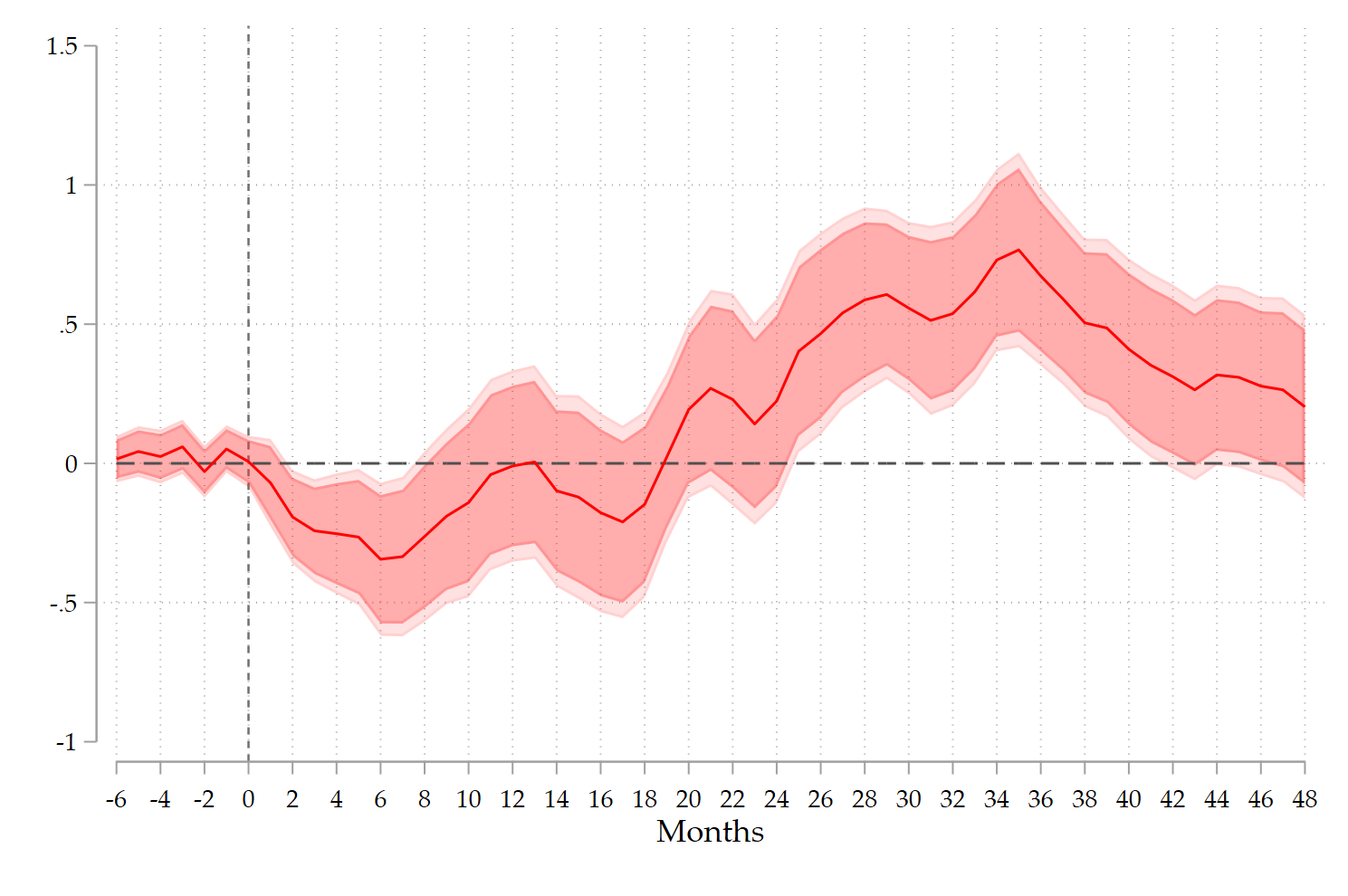
Figure 1. Response of log WTI prices to an instrumented change in geopolitical relations, controlling for the first two future values of the geopolitical turning-point instrument. The dark and light shaded areas represent pointwise 90% and 95% robust confidence intervals.

The lead-augmented estimates reveal a pronounced two-stage response.

No systematic pre-response

All negative-horizon coefficients have 95% confidence intervals containing zero.

The appropriate conclusion is therefore that there is no systematic evidence of pre-response dynamics.

A short-run decline

The impact response is approximately zero:

$$\widehat{\beta}_0=0.006.$$

The response becomes negative and statistically significant at the 5% level from months 2 through 7:

$$\widehat{\beta}_2=-0.193, \qquad 95\%\ CI=[-0.361,-0.024],$$$$\widehat{\beta}_3=-0.242, \qquad 95\%\ CI=[-0.427,-0.057],$$

and the trough occurs at month 6:

$$\widehat{\beta}_6=-0.344, \qquad 95\%\ CI=[-0.619,-0.070].$$

The response remains negative at month 8, where it is significant at the 10% level, and then gradually dissipates.

A delayed positive reversal

The point estimate turns positive around months 19-20. It becomes statistically significant at the 5% level at month 25:

$$\widehat{\beta}_{25}=0.403, \qquad 95\%\ CI=[0.040,0.766].$$

The positive response remains significant through month 41. Its maximum occurs around month 35:

$$\widehat{\beta}_{35}=0.767, \qquad 95\%\ CI=[0.417,1.117].$$

The response subsequently declines, although it remains positive over the rest of the projection window.

How to interpret the vertical axis

Both lwti and lpri are expressed in logs. The LP-IV coefficients are therefore dynamic elasticities.

For example:

$$\widehat{\beta}_6=-0.344$$

means that a 1% instrument-induced increase in the bilateral political-relationship index is associated with an approximately 0.344% decline in WTI prices after six months.

Similarly:

$$\widehat{\beta}_{35}=0.767$$

corresponds to an approximately 0.767% increase in WTI prices after 35 months for a 1% instrument-induced increase in the relationship index.

The coefficients should not be interpreted as a 34.4% decline and a 76.7% increase.

The conditional first stage remains exceptionally strong

The robust conditional first-stage $F$-statistics range from approximately 282 to 414 across the reported positive horizons. The corresponding partial $R^2$ values range from approximately 0.67 to 0.78.

Partialling out the first two future instrument realizations therefore does not create a weak-instrument problem. The sharp change in the estimated dynamic response reflects a change in identifying variation, not a collapse in instrument relevance.

9. Compare the specifications over the same sample

Adding future values of the instrument removes observations from the end of the sample. A valid comparison between the baseline and lead-augmented LP-IV should therefore use the same estimation sample.

First, define the sample for which both future instrument values are observed:

capture drop sample_f2

gen byte sample_f2 =                                   ///
    !missing(F.d2pri) & !missing(F2.d2pri)

Estimate the baseline LP-IV over that sample:

locproj lwti lpri                                      ///
    llwip D.llgop l2lwip D.l2lgop                     ///
    if sample_f2,                                      ///
    h(-12/48) yl(3) sl(2)                              ///
    m(ivregress gmm)                                   ///
    instr(d2pri)                                       ///
    ivtest(firststage)                                 ///
    conf(90 95) r                                      ///
    save irfn(BaselineSame)                            ///
    nograph

Then estimate the lead-augmented specification over exactly the same sample:

locproj lwti lpri F(1/2).d2pri                         ///
    llwip D.llgop l2lwip D.l2lgop                     ///
    if sample_f2,                                      ///
    h(-12/48) yl(3) sl(2)                              ///
    m(ivregress gmm)                                   ///
    instr(d2pri)                                       ///
    ivtest(firststage)                                 ///
    conf(90 95) r                                      ///
    save irfn(TZ2Same)                                 ///
    nograph

The two point estimates can be plotted on a common axis:

lpgraph BaselineSame TZ2Same,                            ///
    hor(-12/48)                                          ///
    zero                                                 ///
    tti(Months)                                          ///
    lab1("Baseline LP-IV")                               ///
    lab2("Two future-instrument controls")               ///
    lc1(navy) lc2(red)                                   ///
    title("Baseline and Lead-Augmented LP-IV Responses") ///
    grname(Figure_comparison)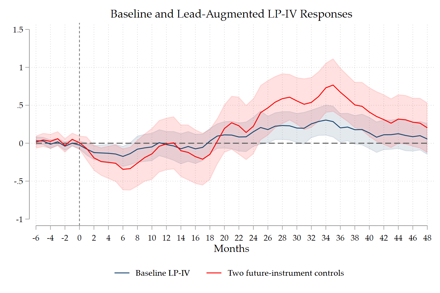

Figure 2. Comparisons of response of log WTI prices to an instrumented change in geopolitical relations, without (blue) and with (red) controlling for the first two future values of the geopolitical turning-point instrument. The dark and light shaded areas represent pointwise 95% robust confidence intervals.

This comparison isolates the effect of changing the conditioning set from the mechanical effect of losing terminal observations.

10. Conclusion

The discussion with Davide Romelli at the SILVAPLANA POLITICAL ECONOMY 2026 workshop led to a simple but consequential modification of the LP-IV specification.

The Teulings-Zubanov insight is that events occurring after the initial shock can affect the outcome inside the local-projection horizon. When these subsequent events are related to the original shock, omitting them can cause the estimated response to incorporate an entire sequence of events.

In an LP-IV setting, future values of the endogenous impulse cannot generally be added as ordinary exogenous controls. A practical adaptation is instead to retain the contemporaneous external instrument as the excluded instrument and treat its future values as included controls.

The resulting LP-IV identifies the response using contemporaneous instrument variation orthogonal to those future realizations.

In the oil-price application, controlling for the first two future geopolitical turning points produces:

• no systematic pre-response;
• a statistically significant decline in WTI prices from months 2 through 7;
• a trough at approximately month 6;
• a delayed positive reversal that is significant from months 25 through 41;
• an exceptionally strong conditional first stage.

The baseline LP-IV is closer to the response associated with the geopolitical sequence that normally follows the initial turning point. The lead-augmented LP-IV is closer to the response to a contemporaneous instrument innovation after holding its first two future realizations fixed.

That distinction is the broader lesson. In dynamic causal analysis, selecting an external instrument is only one part of the identification problem. Researchers must also decide which future shock path is embedded in the impulse response they want to estimate.

References

Alloza, M., Gonzalo, J., and Sanz, C. (2025). “Dynamic Effects of Persistent Shocks.” Journal of Applied Econometrics, 40(4), 380-394.

Jordà, Ò. (2005). “Estimation and Inference of Impulse Responses by Local Projections.” American Economic Review, 95(1), 161-182.

Jordà, Ò., and Taylor, A. M. (2025). “Local Projections.” Journal of Economic Literature, 63(1), 59-110.

Montiel Olea, J. L., and Plagborg-Møller, M. (2021). “Local Projection Inference Is Simpler and More Robust Than You Think.” Econometrica, 89(4), 1789-1823.

Stock, J. H., and Watson, M. W. (2018). “Identification and Estimation of Dynamic Causal Effects in Macroeconomics Using External Instruments.” Economic Journal, 128(610), 917-948.

Teulings, C. N., and Zubanov, N. (2014). “Is Economic Recovery a Myth? Robust Estimation of Impulse Responses.” Journal of Applied Econometrics, 29(3), 497-514.

Ugarte-Ruiz, A. (2025). “Locproj and Lpgraph: Stata Commands to Estimate Local Projections.” BBVA Research Working Paper 25/09.