I am currently attending the Timberlake Econometrics Summer School at Churchill College, Cambridge, where I am following Professor Jeffrey Wooldridge’s class. This course provided an excellent opportunity to revisit my earlier blog post on heterogeneous difference-in-differences with Stata.
In this post, I compare four Stata implementations of regression adjustment for staggered difference-in-differences:
- Stata’s official
xthdidregress racommand; - the transformation-based
lwdidcommand developed by Soo Jeong Lee and Jeffrey Wooldridge; - the saturated-regression implementation available through
jwdid; - the regression-adjustment implementation available through
csdid.
The objective is deliberately narrow. I estimate the same regression-adjustment model with all four commands. I do not compare regression adjustment with AIPW, IPWRA, doubly robust estimators, or other extended two-way fixed-effects specifications, because those exercises would involve different estimators and would not generally produce identical estimates.
The main result is clear: once the estimation sample, covariates, control group, treatment cohorts, reference period, clustering level, and aggregation weights are aligned, all four commands produce numerically identical point estimates. Their standard errors and confidence intervals need not coincide because the commands use different computational and inference procedures.
The minimum-wage application
I use the same minwage dataset as in my original blog. It contains a balanced panel of 2,284 counties observed annually between 2001 and 2007:
The outcome variable, lemp, is the logarithm of county employment. Treatment occurs at the state level, with treatment cohorts beginning in 2004, 2006, and 2007. Counties in states that are never treated provide the comparison group.
The covariate specification is unchanged:
global covars i.region pop medinc white hs pov c.pop#c.pop ///
    c.medinc#c.medinc
It includes region indicators, population, median income, demographic and educational variables, poverty, and quadratic terms for population and median income.
The county is the panel unit, but treatment is assigned at the state level. Accordingly, the estimation uses countyreal as the panel identifier and clusters inference at the state level. There are 29 state clusters.
The regression-adjustment estimator
For each treatment cohort and calendar year , define the change relative to the last pretreatment year:
Regression adjustment uses the never-treated observations to estimate the expected untreated change conditional on the covariates:
The cohort-time treatment effect is obtained by averaging the difference between the observed change and the estimated counterfactual change among the units belonging to cohort :
Regression adjustment is not doubly robust. Its validity depends on the usual difference-in-differences assumptions—including no anticipation and conditional parallel trends—as well as an appropriately specified outcome regression.
Estimation with xthdidregress
The first estimator is:
local reps 999
local seed 271828

xthdidregress ra (lemp $covars) (treat), ///
    group(state) controlgroup(never) basetime(common)
Two options deserve particular attention.
First, controlgroup(never) makes the never-treated comparison group explicit. This is already the default for xthdidregress, but stating it explicitly helps align the two commands.
Second, basetime(common) uses , the final pretreatment period, as the reference year for every pretreatment and post-treatment estimate.
By default, xthdidregress uses an adaptive reference period before treatment: a pretreatment effect for year compares with . Post-treatment effects always use . The common-base option therefore changes the presentation of the pretreatment coefficients but leaves all post-treatment estimates unchanged. This distinction is explained in the xthdidregress documentation.
I save the estimation sample so that lwdid uses exactly the same observations:
tempvar sample_ra
generate byte `sample_ra' = e(sample)
The overall and event-time effects are obtained as follows:
estat aggregation, overall weights(timecohort)

estat aggregation, dynamic weights(timecohort) ///
    sci(reps(`reps') rseed(`seed')) ///
    graph(name(d1, replace))

graph export "figures\event.png", as(png) ///
    name("d1") replace
The weights(timecohort) option weights the contributing cohort-time effects by the number of treated observations in each cell. The sci() option requests simultaneous rather than pointwise confidence intervals.
The equivalent specification with lwdid
The lwdid command implements the transformation-based rolling difference-in-differences estimators developed by Lee and Wooldridge. It can be installed from SSC:
ssc install lwdid, replaceBefore estimation, I use fvrevar to expand the factor-variable and quadratic terms used in the original model:
fvrevar $covars
local covars_lwdid "`r(varlist)'"
This does not change the model. It simply converts expressions such as i.region, c.pop#c.pop, and c.medinc#c.medinc into the corresponding numeric variables required by lwdid.
The aligned regression-adjustment specification is:
lwdid lemp `covars_lwdid' if `sample_ra', ///
    ivar(countyreal) tvar(year) gvar(_did_cohort) ///
    rolling(demean) pre(1) method(ra) never ///
    cluster(state) attgt graph level(95) ///
    reps(`reps') seed(`seed') ///
    gopts(name(lwdid_event, replace))

graph export "figures\lwdid_event.png", as(png) ///
    name("lwdid_event") replace
The correspondence between the options is important:
ivar(countyreal)identifies the county panel.tvar(year)identifies calendar time.gvar(_did_cohort)uses the cohort variable constructed byxthdidregress.neverrestricts the comparison group to never-treated states.cluster(state)clusters inference at the treatment-assignment level.method(ra)selects regression adjustment.rolling(demean) pre(1)subtracts the final pretreatment outcome.
With pre(1), the pretreatment mean contains only one observation. Therefore, demeaning is simply:
This is precisely the transformation used by xthdidregress ra with basetime(common). More details about this transformation approach are available in Lee and Wooldridge and the lwdid documentation.
Extending the comparison to jwdid and csdid
The same regression-adjustment estimand can also be recovered through two additional Stata implementations.
First, jwdid estimates the fully saturated regression representation. Second, csdid implements the regression-adjustment version of the Callaway–Sant’Anna estimator. To make the comparison meaningful, I continue to use:
- the exact estimation sample selected by
xthdidregress; - the same outcome and covariates;
- the same treatment cohorts;
- never-treated states as the comparison group;
- the common g−1 reference period;
- counties as the panel units;
- state-level clustering.
The four aligned specifications are therefore:
| Command | Aligned specification |
|---|---|
xthdidregress | ra, controlgroup(never), basetime(common) |
lwdid | rolling(demean) pre(1) method(ra) never |
jwdid | never |
csdid | method(reg) long2 |
The saturated regression with jwdid
The jwdid specification is:
jwdid lemp $covars if `sample_ra',                     ///
    ivar(countyreal) tvar(year) gvar(_did_cohort)      ///
    never cluster(state)

estat attgt
estat simple
estat event
estat group
estat calendar
The never option is essential. It restricts the control group to never-treated states, matching the comparison group used by the other three implementations.
Unlike xthdidregress, which estimates the relevant outcome regressions separately, jwdid recovers the treatment effects from one very long saturated regression. The output contains interactions between treatment cohorts, calendar years, treatment status, and the covariates. This explains the length of the underlying regression table.
In this application, some saturated interactions are omitted because of collinearity, and jwdid also reports warnings related to singleton observations and the limited number of state clusters. These warnings do not alter the recovered treatment-effect point estimates, which coincide with the other implementations, but the command-specific inferential output should be interpreted cautiously.
Regression adjustment with csdid
The equivalent csdid specification is:
csdid lemp $covars if `sample_ra',                     ///
    ivar(countyreal) time(year) gvar(_did_cohort)      ///
    method(reg) long2 cluster(state)

estat attgt
estat simple
estat event
estat group
estat calendar
Two options are particularly important.
The method(reg) option selects regression adjustment. Without it, csdid uses a different default estimator and the exercise would no longer be a comparison of identical regression-adjustment specifications.
The long2 option constructs the pretreatment comparisons relative to the common final pretreatment period, g−1. It therefore aligns the reference period with xthdidregress, basetime(common), lwdid, pre(1), and jwdid, never.
Four implementations, identical point estimates
The four commands return the same post-treatment cohort-time effects. Consequently, the event-time point estimates are also identical:
| Exposure time | Common estimate | Exact employment effect |
|---|---|---|
| 0 | −0.0245258 | −2.42% |
| 1 | −0.0524273 | −5.11% |
| 2 | −0.0751323 | −7.24% |
| 3 | −0.0840835 | −8.06% |
The common weighted overall post-treatment estimate is:
Because the outcome is the logarithm of employment, the corresponding exact percentage effect is:
Thus, all four computational representations imply an average employment decline of approximately 3.8% following treatment.
The Stata results confirm that jwdid returns the same overall estimate and the same event-time coefficients as the other implementations. Its delta-method standard error for the overall effect is 0.0074471.
csdid, method(reg) long2 also returns an overall estimate of −0.0385318. Its standard error, 0.0111631, is exactly the same as the corresponding xthdidregress standard error in this application.
A clarification concerning csdid’s Post_avg
After estat event, csdid additionally reports:
Post_avg = -0.0590422This is not the same aggregation as the treated-observation-weighted overall effect. It is the arithmetic mean of the four reported post-treatment event-time coefficients:
The relevant comparison with the overall effects from the other commands is therefore:
estat simplewhich returns −0.0385318. The Post_avg from csdid’s event aggregation should not be compared directly with xthdidregress, weights(timecohort) or the baseline lwdid weighted post-treatment average.
Four-way event-study comparison
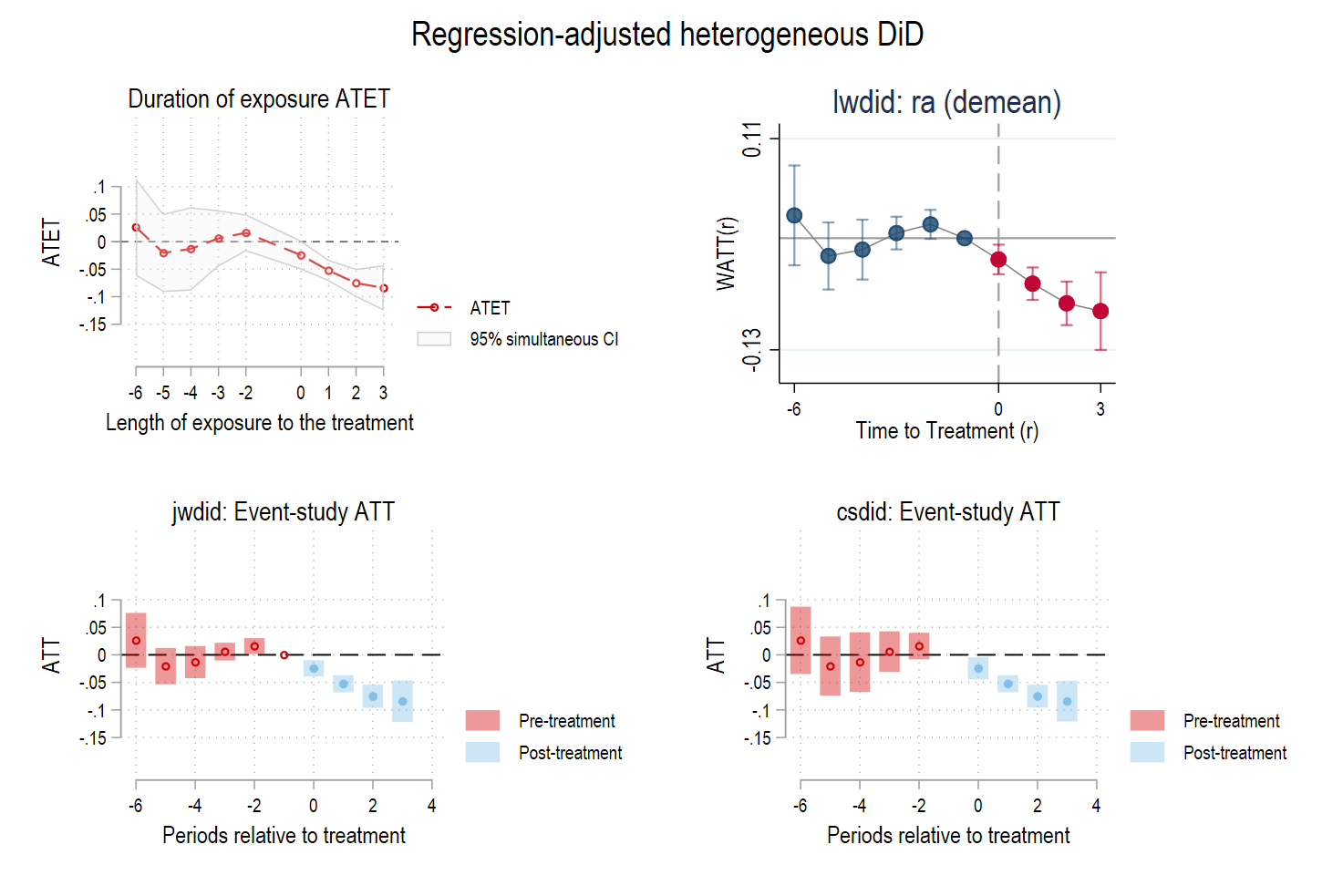
Figure 1. Regression-adjusted event-study estimates from xthdidregress, lwdid, jwdid, and csdid. The four implementations produce identical event-time point estimates after aligning the sample, covariates, control group, reference period, and aggregation. The confidence intervals should not be compared as though they were constructed identically: the xthdidregress and lwdid panels display simultaneous confidence bands, whereas the native jwdid and csdid graphs display pointwise intervals. Exposure −1 is the common reference period.
The figure provides a direct visual demonstration of point-estimate equivalence. All four paths move from estimates close to zero before treatment to progressively more negative effects after treatment.
The visual differences concern the uncertainty intervals rather than the estimates themselves. In particular, the first two panels use simultaneous inference over the event-study path, while the last two report their native pointwise intervals.
Cohort-specific effects
The cohort aggregations produced by xthdidregress, jwdid, and csdid are also numerically identical:
| Treatment cohort | Common estimate |
|---|---|
| 2004 | −0.0639002 |
| 2006 | −0.0288356 |
| 2007 | −0.0285611 |
The earliest-treated cohort has the largest average decline in employment. This cohort is observed for four post-treatment periods, whereas the 2007 cohort is observed only in its treatment year. The difference across cohorts therefore combines treatment-effect heterogeneity with differences in the available post-treatment horizons.
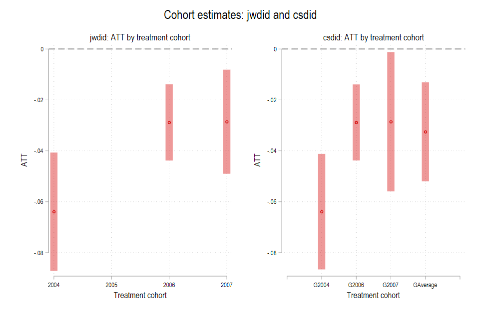
Figure 2. Treatment-cohort aggregations from jwdid and csdid. The estimates for the 2004, 2006, and 2007 cohorts are identical. The csdid panel additionally reports GAverage, a separate average across treatment groups; it has no corresponding cohort point in the jwdid panel.
The reported jwdid cohort estimates are −0.0639002, −0.0288356, and −0.0285611. csdid returns the same three-point estimates, although the commands attach different standard errors to some of them.
Calendar-time effects
The calendar-time aggregations are likewise identical:
| Calendar year | Common estimate |
|---|---|
| 2004 | −0.0415691 |
| 2005 | −0.0548160 |
| 2006 | −0.0276208 |
| 2007 | −0.0402872 |
The effect is most negative in 2005. The 2006 estimate is smaller in absolute value because it combines the relatively large negative effect for the 2004 cohort with the near-zero impact estimate for the cohort first treated in 2006.
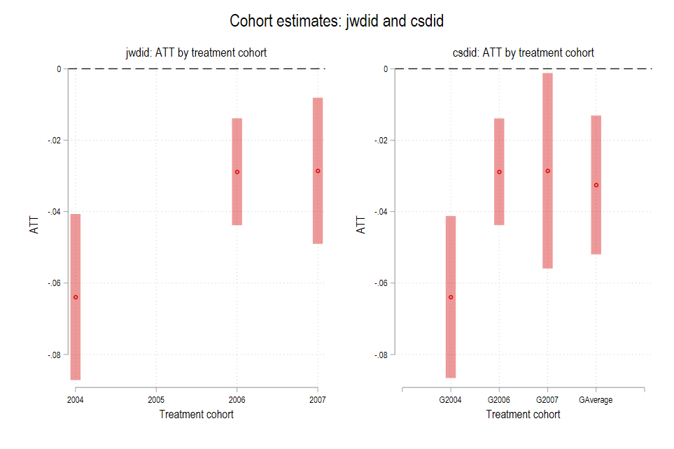
Figure 3. Calendar-time aggregations from jwdid and csdid. The point estimates for 2004–2007 coincide exactly. The csdid panel additionally displays CAverage, an average over the calendar-time effects rather than a separate calendar year.
The common calendar-year point estimates are visible in both outputs, although the confidence intervals differ because the variance estimators are not identical.
Point estimates versus inference
The overall comparison is:
| Command | Overall estimate | Standard error | 95% pointwise interval |
|---|---|---|---|
xthdidregress ra | −0.0385318 | 0.0111631 | [−0.0604111, −0.0166525] |
lwdid, method(ra) | −0.0385318 | 0.0071951 | [−0.0526340, −0.0244296] |
jwdid, never | −0.0385318 | 0.0074471 | [−0.0531279, −0.0239357] |
csdid, method(reg) long2 | −0.0385318 | 0.0111631 | [−0.0604111, −0.0166525] |
The equality of the point estimates is exact up to the displayed numerical precision. The equality of standard errors is not general. In this application, xthdidregress and csdid return the same standard error for the overall effect, while the transformed lwdid calculation and the saturated jwdid regression produce smaller but slightly different standard errors.
The four-way figure should therefore be read as evidence about the estimated path, not as a comparison of four interchangeable confidence procedures.
What does the four-command comparison establish?
After aligning the estimation sample, covariates, treatment cohorts, never-treated comparison group, common g−1 reference period, clustering level, and aggregation weights, xthdidregress ra, lwdid, method(ra), jwdid, never, and csdid, method(reg) long2 recover the same regression-adjusted cohort-time, event-time, and overall treatment-effect point estimates in this minimum-wage application.
The result is not that the four commands are universally interchangeable. Their default comparison groups, transformations, reference periods, aggregation rules, and inferential procedures differ. Equivalence emerges only after the complete estimand has been aligned.
Graphical comparison
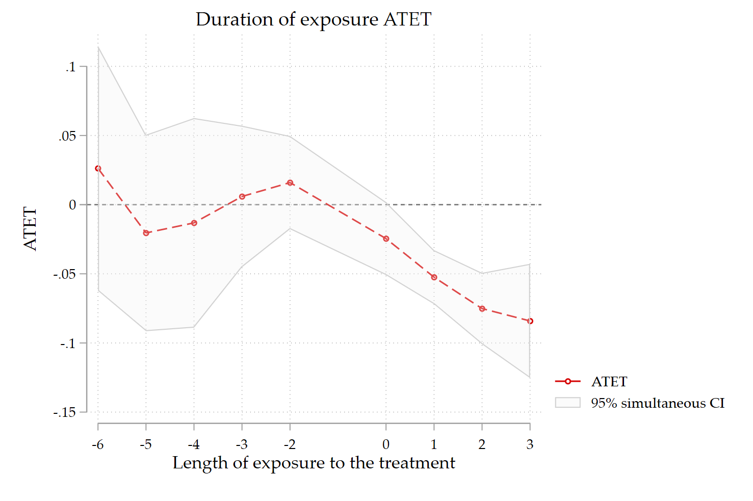
Figure 4. Event-time ATETs estimated with xthdidregress ra. The dashed red line reports the point estimates, while the grey envelope shows the 95% simultaneous confidence intervals. Exposure −1 is the common reference period and is omitted.
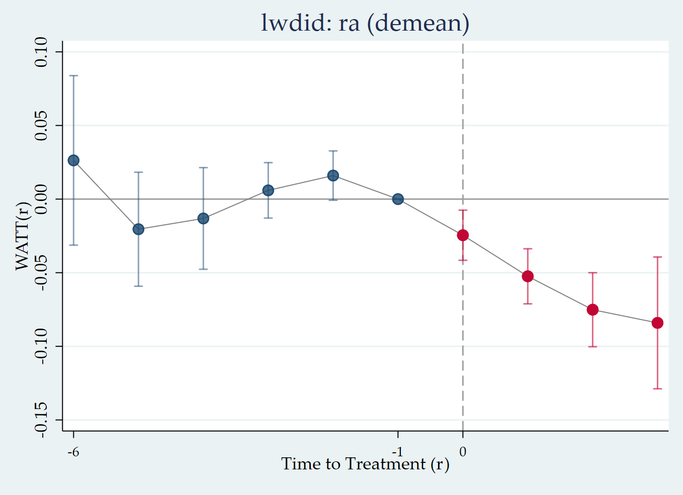
Figure 5. Event-time WATT(r) estimates obtained with lwdid, method(ra). Pretreatment estimates are shown in blue and post-treatment estimates in red. The vertical intervals are 95% simultaneous confidence bands. Exposure −1 is normalized to zero.
This overall estimate is not the simple arithmetic mean of the four event-time coefficients. It is a treated-observation-weighted average of the seven available post-treatment cells.
The composition of the event-time estimates also changes with the horizon. At exposure zero, all three treatment cohorts contribute. At exposure one, only the 2004 and 2006 cohorts contribute. At exposures two and three, only the 2004 cohort remains observable. The increasingly negative dynamic path should therefore be interpreted with this changing cohort composition in mind.
Why are the confidence intervals different?
Identical point estimates do not imply identical inference.
For the overall effect, the commands report:
| Command | Estimate | Standard error | 95% pointwise interval |
|---|---|---|---|
xthdidregress | −0.0385318 | 0.0111631 | [−0.0604111, −0.0166525] |
lwdid | −0.0385318 | 0.0071951 | [−0.0526340, −0.0244296] |
Stata’s sci() option constructs multiplier-bootstrap simultaneous intervals. The lwdid event graph uses its own clustered wild-bootstrap procedure. Consequently, using the same number of replications and the same random-number seed does not make the confidence bands identical.
The difference is particularly visible at exposure zero:
- the
xthdidregresssimultaneous interval is [−0.05096, 0.00191]; - the
lwdidsimultaneous band is [−0.04155, −0.00750].
The first includes zero, while the second does not. From exposure one to exposure three, both procedures produce simultaneous bands that exclude zero.
All the pretreatment simultaneous bands include zero under both procedures. Moreover, lwdid reports:
This is reassuring, but it should not be overinterpreted. Pre_avg is an average of pretreatment effects, not a joint test that every individual lead equals zero. More generally, a failure to reject pretreatment effects does not prove that parallel trends holds.
It is also important to distinguish the pointwise p-values displayed by lwdid from the simultaneous confidence bands shown in its event-study graph. A pointwise p-value may be below 5% even when the corresponding simultaneous band contains zero because the simultaneous band accounts for inference across the entire event-time path.
Robustness: lags-only and detrended specifications
After I shared the initial results on LinkedIn, Professor Jeffrey Wooldridge suggested two additional robustness checks.
First, he recommended dropping pre(1). The baseline specification uses only , the final pretreatment period, to construct the reference outcome. Without pre(1), lwdid instead uses all available pretreatment periods. This produces the Lee–Wooldridge “lags-only” estimator.
Second, he recommended replacing rolling(demean) with rolling(detrend). This examines whether the results are robust to removing unit-specific linear trends before estimating the treatment effects.
These two exercises follow the intended comparison exactly: both use all available pretreatment periods, and the second changes only the transformation from demeaning to detrending. The official lwdid documentation confirms that omitting pre() uses all available pretreatment observations. Professor Wooldridge provides a useful discussion of the distinction between the transformations on Statalist.
Lags only: using all pretreatment periods
The first robustness check is:
lwdid lemp `covars_lwdid' if `sample_ra',             ///
    ivar(countyreal) tvar(year) gvar(_did_cohort)     ///
    rolling(demean) method(ra) never                  ///
    cluster(state) attgt graph level(95)              ///
    reps(`reps') seed(`seed')                         ///
    gopts(name(lwdid_lags, replace))

graph export "figures\lwdid_lags.png", as(png)        ///
    name("lwdid_lags") replace
The absence of pre() is deliberate. For treatment cohort , the transformed outcome now subtracts the unit-specific average over all available periods preceding treatment:
“Lags only” refers to the construction of the post-treatment effects. The command still reports separately constructed pretreatment placebo estimates for diagnostic purposes.
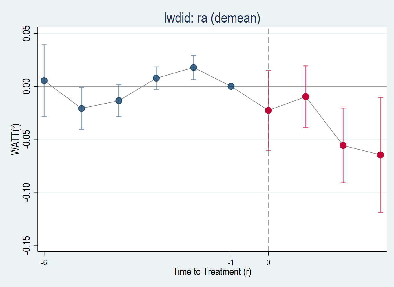
Figure 3. Lags-only regression-adjustment estimates obtained with rolling(demean) and all available pretreatment periods. Pretreatment estimates appear in blue and post-treatment estimates in red. The intervals are 95% simultaneous confidence bands. Exposure −1 is normalized to zero.
Allowing for unit-specific linear trends
The second robustness check changes only the transformation:
lwdid lemp `covars_lwdid' if `sample_ra',             ///
    ivar(countyreal) tvar(year) gvar(_did_cohort)     ///
    rolling(detrend) method(ra) never                 ///
    cluster(state) attgt graph level(95)              ///
    reps(`reps') seed(`seed')                         ///
    gopts(name(lwdid_detrend, replace))

graph export "figures\lwdid_detrend.png", as(png)     ///
    name("lwdid_detrend") replace
For each unit and treatment cohort, rolling(detrend) estimates a linear trend using the available pretreatment observations:
and constructs the detrended outcome:
This permits treatment timing to be related to unit-specific linear untreated trends. It therefore relaxes the standard parallel-trends assumption in an important direction. However, it replaces that assumption with a linear-trend structure and extrapolates the estimated pretreatment trend into the post-treatment period.
This qualification matters here because the earliest cohort, treated in 2004, has only three pretreatment observations: 2001, 2002, and 2003.
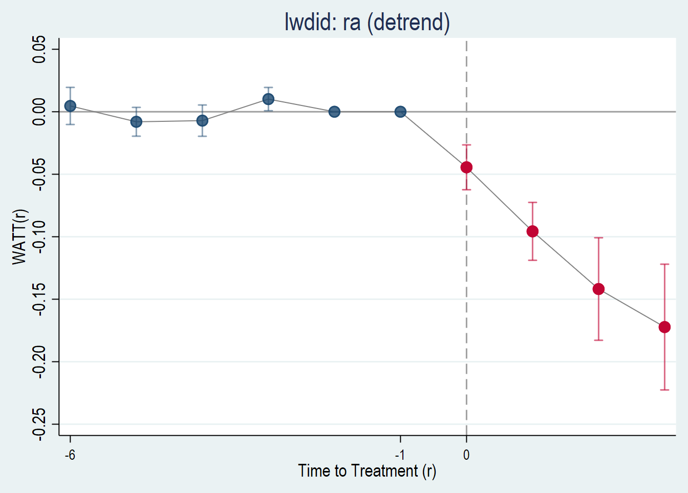
Figure 4. Regression-adjustment estimates after removing unit-specific linear pretreatment trends. The intervals are 95% simultaneous confidence bands. Under the detrended placebo construction, exposures −2 and −1 are normalized to zero and should not be interpreted as estimated evidence in favor of parallel trends.
Comparison of the weighted average effects
The three specifications produce the following weighted post-treatment averages:
| Specification | Post_avg | Standard error | Pointwise p-value | Exact employment effect |
|---|---|---|---|---|
Baseline: demean pre(1) | −0.03853 | 0.00720 | <0.001 | −3.78% |
Lags only: demean | −0.02509 | 0.01248 | 0.044 | −2.48% |
Detrended: detrend | −0.07176 | 0.00721 | <0.001 | −6.92% |
The exact employment effects use:
The estimated weighted average remains negative under all three transformations. Nevertheless, its magnitude is sensitive to the treatment of the pretreatment outcomes: the exact employment effect ranges from approximately −2.48% under lags-only demeaning to −6.92% after detrending.
How costly is using all pretreatment periods?
Dropping pre(1) reduces the absolute magnitude of the weighted average estimate from 0.0385 to 0.0251. More importantly, its standard error increases from 0.00720 to 0.01248—an increase of approximately 73%.
Thus, using all available pretreatment periods does not improve precision in this application. The pointwise p-value of the weighted average rises from below 0.001 to 0.044.
There is no mechanical guarantee that averaging more pretreatment observations will reduce the sampling uncertainty of the final ATT estimate. The result also depends on the time-series dependence of the outcome, the distance between the earlier pretreatment observations and treatment, and the covariance among the contributing cohort-time estimates.
Is detrending costly in terms of precision?
For the single weighted average effect, the answer is clearly no.
Replacing demeaning with detrending reduces the standard error from 0.01248 to 0.00721, a decline of approximately 42%. The detrended standard error is also almost identical to the baseline pre(1) standard error: it is only 0.3% larger.
The precision comparison is not uniform at every exposure time. Relative to lags-only demeaning, detrending lowers the standard errors at exposures 0, 1, and 3, but raises the standard error at exposure 2 by approximately 16%. The conclusion that detrending improves precision therefore applies to the single weighted average—not to every underlying effect.
Comparison of the dynamic effects
The event-time estimates and their standard errors are:
| Exposure | Baseline: demean pre(1) | Lags only: demean | Detrended: detrend |
|---|---|---|---|
| 0 | −0.02453 (0.00727) | −0.02278 (0.01510) | −0.04444 (0.00719) |
| 1 | −0.05243 (0.00799) | −0.00978 (0.01167) | −0.09568 (0.00929) |
| 2 | −0.07513 (0.01073) | −0.05583 (0.01415) | −0.14182 (0.01645) |
| 3 | −0.08408 (0.01911) | −0.06478 (0.02177) | −0.17227 (0.02017) |
Note: Standard errors are reported in parentheses.
Under lags-only demeaning, the estimated effects at exposures 0 and 1 are relatively small and their simultaneous confidence bands include zero. The effects become clearly negative only at exposures 2 and 3.
Detrending produces a much stronger negative path. The exact employment effects range from approximately −4.35% on impact to −15.82% after three years, and all four post-treatment simultaneous bands exclude zero.
This difference is not a uniform rescaling. For example, the 2006 cohort’s impact estimate changes from +0.0468 under demeaning to −0.0248 after detrending. Its one-year effect changes from approximately zero to −0.0937. The 2004 cohort also becomes substantially more negative, whereas the impact estimate for the 2007 cohort changes very little.
At exposures 2 and 3, only the 2004 cohort remains observable. The large long-run detrended estimates therefore combine the transformation’s effect with the changing composition of the event-time aggregation.
What happens to the pretreatment diagnostics?
The average pretreatment effects are almost exactly zero:
| Specification | Pre_avg | Standard error | Pointwise p-value |
|---|---|---|---|
Lags only: demean | −0.00039 | 0.00210 | 0.851 |
Detrended: detrend | −0.00009 | 0.00090 | 0.924 |
These averages conceal some individual deviations.
Under lags-only demeaning, the simultaneous confidence bands exclude zero at exposures −5 and −2. Under detrending, the simultaneous band excludes zero at exposure −3. The remaining detrended placebo estimates at −6, −5, and −4 include zero.
The detrended values at −2 and −1 are zero by construction. Moreover, the detrended Pre_avg is computed only from the earlier estimable placebo periods. These zeros must therefore not be treated as evidence supporting the identifying assumptions.
As in the baseline analysis, Pre_avg is an average rather than a joint test of every pretreatment coefficient. A near-zero average can arise because positive and negative deviations offset one another.
Conclusion: What does this exercise establish?
This application shows that regression-adjusted heterogeneous difference-in-differences can be represented in several computationally distinct ways: through cohort-time outcome regressions, transformed rolling differences, a saturated levels regression, or the Callaway–Sant’Anna regression-adjustment implementation. Once the complete estimand is aligned, all four approaches recover the same point estimates.
The exercise also illustrates why numerical replication should proceed in stages. Researchers should first verify the cohort-time effects, then the aggregation weights, and only afterward compare standard errors and confidence intervals. Agreement in point estimates establishes that the same estimand has been recovered; disagreement in inference may simply reflect different variance estimators, bootstrap procedures, or degrees-of-freedom corrections.
References
Callaway, B., and P. H. C. Sant’Anna. 2021. “Difference-in-Differences with Multiple Time Periods.” Journal of Econometrics 225(2): 200–230.
Lee, S. J., and J. M. Wooldridge. “A Simple Transformation Approach to Difference-in-Differences Estimation for Panel Data.”
Lee, S. J., and J. M. Wooldridge. “LWDID: Rolling Difference-in-Differences Estimator for Small-N and Large-N Panel Data.” Statistical Software Components.
StataCorp. xthdidregress: Heterogeneous Difference-in-Differences for Panel Data.
Full code
// Clear the console and the data

cls
clear
graph drop _all

// Change the folder for the current directory

cd "C:\Users\jamel\Dropbox\stata\hdidweb"

// Open a log

capture log close
log using hdidweb_ra_lwdid_csdid_jwdid_plots.log, replace text

// Use the same data as in the blog

use minwage

describe
xtdescribe

sum
xtsum

capture mkdir "figures"

// Use the exact covariate specification from the blog

global covars i.region pop medinc white hs pov c.pop#c.pop  ///
    c.medinc#c.medinc

// Use the same replications and seed for the simultaneous-band procedures

local reps 999
local seed 271828

// -----------------------------------------------------------------------------
// 1. xthdidregress: regression adjustment
// -----------------------------------------------------------------------------

// basetime(common) uses g-1 for all pretreatment comparisons.
// This is the only change needed to align the full event-study path with
// lwdid, pre(1). It does not change the post-treatment estimates.

xthdidregress ra (lemp $covars) (treat),                  ///
    group(state) controlgroup(never) basetime(common)

// Keep exactly the same estimation sample for all alternative commands

tempvar sample_ra
generate byte `sample_ra' = e(sample)

// Plot the cohort-time ATETs with simultaneous 95% confidence bands

estat atetplot, sci(reps(`reps') rseed(`seed'))           ///
    name(atet, replace)
graph export "figures\atetplot.png", as(png)             ///
    name("atet") replace

// Overall post-treatment ATET
// This is directly comparable with Post_avg reported by lwdid.

estat aggregation, overall weights(timecohort)

// Event study with simultaneous 95% confidence bands

estat aggregation, dynamic weights(timecohort)            ///
    sci(reps(`reps') rseed(`seed'))                       ///
    graph(name(d1, replace))
graph export "figures\event.png", as(png)                ///
    name("d1") replace

// ATETs over cohort

estat aggregation, cohort graph(name(c1, replace))
graph export "figures\cohort.png", as(png)               ///
    name("c1") replace

// ATETs across calendar time

estat aggregation, time graph(name(t1, replace))
graph export "figures\time.png", as(png)                 ///
    name("t1") replace

// -----------------------------------------------------------------------------
// 2. lwdid: the equivalent regression-adjustment specification
// -----------------------------------------------------------------------------

// lwdid requires numeric covariates. fvrevar expands the factor-variable
// terms without changing the covariate specification. Keep this expanded
// list only for lwdid; jwdid and csdid accept the original FV notation.

fvrevar $covars
local covars_lwdid "`r(varlist)'"

// _did_cohort is created above by xthdidregress from treat and state.
// All four implementations therefore use the same sample, cohorts, controls,
// covariates, reference period, treatment level, and clustering level.

lwdid lemp `covars_lwdid' if `sample_ra',                 ///
    ivar(countyreal) tvar(year) gvar(_did_cohort)         ///
    rolling(demean) pre(1) method(ra) never               ///
    cluster(state) attgt graph level(95)                  ///
    reps(`reps') seed(`seed')                             ///
    gopts(name(lwdid_event, replace))

// The native lwdid event-study graph contains simultaneous 95% bands.

graph export "figures\lwdid_event.png", as(png)          ///
    name("lwdid_event") replace

// -----------------------------------------------------------------------------
// 3. jwdid: saturated-regression representation
// -----------------------------------------------------------------------------

// never restricts the comparison group to never-treated units.
// jwdid accepts factor-variable notation directly. Using $covars here avoids
// passing fvrevar's temporary __00000# variables to jwdid/hdfe, which causes
// r(198) when those variables are expanded again internally.

jwdid lemp $covars if `sample_ra',                        ///
    ivar(countyreal) tvar(year) gvar(_did_cohort)         ///
    never cluster(state)

// Cohort-time ATT estimates: the most direct numerical comparison.
// jwdid's plotting routine does not draw the complete ATT(g,t) table, so the
// figures below are generated from the event, group, and calendar aggregations.

estat attgt

// Overall post-treatment ATT

estat simple

// Event-time ATT estimates and plot. estat plot must immediately follow the
// aggregation whose r() results are to be plotted.

estat event
estat plot, name(jwdid_event, replace)                    ///
    title("jwdid: Event-study ATT")                       ///
    ytitle("ATT") xtitle("Periods relative to treatment")
graph export "figures\jwdid_event.png", as(png)          ///
    name("jwdid_event") replace

// ATT estimates by treatment cohort and plot

estat group
estat plot, name(jwdid_group, replace)                    ///
    title("jwdid: ATT by treatment cohort")               ///
    ytitle("ATT") xtitle("Treatment cohort")
graph export "figures\jwdid_group.png", as(png)          ///
    name("jwdid_group") replace

// ATT estimates by calendar time and plot

estat calendar
estat plot, name(jwdid_calendar, replace)                 ///
    title("jwdid: ATT by calendar time")                  ///
    ytitle("ATT") xtitle("Calendar year")
graph export "figures\jwdid_calendar.png", as(png)       ///
    name("jwdid_calendar") replace

// -----------------------------------------------------------------------------
// 4. csdid: Callaway-Sant'Anna regression adjustment
// -----------------------------------------------------------------------------

// method(reg) selects regression adjustment rather than the default doubly
// robust estimator. long2 uses the universal g-1 reference period for the
// pretreatment comparisons. csdid accepts factor-variable notation directly
// and uses never-treated controls by default when they are available.

csdid lemp $covars if `sample_ra',                        ///
    ivar(countyreal) time(year) gvar(_did_cohort)         ///
    method(reg) long2 cluster(state)

// Cohort-time ATT estimates: the most direct numerical comparison.
// A csdid ATT(g,t) plot requires group(#), so the comparable aggregate plots
// are generated below after event, group, and calendar postestimation.

estat attgt

// Overall post-treatment ATT

estat simple

// Event-time ATT estimates and plot. csdid_plot must immediately follow
// estat event so that it uses the event-study results left in r().

estat event
csdid_plot, name(csdid_event, replace)                    ///
    title("csdid: Event-study ATT")                       ///
    ytitle("ATT") xtitle("Periods relative to treatment")
graph export "figures\csdid_event.png", as(png)          ///
    name("csdid_event") replace

// ATT estimates by treatment cohort and plot

estat group
csdid_plot, name(csdid_group, replace)                    ///
    title("csdid: ATT by treatment cohort")               ///
    ytitle("ATT") xtitle("Treatment cohort")
graph export "figures\csdid_group.png", as(png)          ///
    name("csdid_group") replace

// ATT estimates by calendar time and plot

estat calendar
csdid_plot, name(csdid_calendar, replace)                 ///
    title("csdid: ATT by calendar time")                  ///
    ytitle("ATT") xtitle("Calendar year")
graph export "figures\csdid_calendar.png", as(png)       ///
    name("csdid_calendar") replace

// Pairwise graphical comparisons of the jwdid and csdid aggregations

graph combine jwdid_event csdid_event, rows(1) ycommon   ///
    name(jwdid_csdid_event, replace)                      ///
    title("Event-study estimates: jwdid and csdid")
graph export "figures\jwdid_csdid_event.png", as(png)   ///
    name("jwdid_csdid_event") replace

graph combine jwdid_group csdid_group, rows(1) ycommon   ///
    name(jwdid_csdid_group, replace)                      ///
    title("Cohort estimates: jwdid and csdid")
graph export "figures\jwdid_csdid_group.png", as(png)   ///
    name("jwdid_csdid_group") replace

graph combine jwdid_calendar csdid_calendar, rows(1)     ///
    ycommon name(jwdid_csdid_calendar, replace)           ///
    title("Calendar-time estimates: jwdid and csdid")
graph export "figures\jwdid_csdid_calendar.png",        ///
    as(png) name("jwdid_csdid_calendar") replace

// Four-way event-study comparison. The first two graphs use simultaneous
// bands, whereas jwdid and csdid display their native pointwise intervals.

graph combine d1 lwdid_event jwdid_event csdid_event,    ///
    rows(2) ycommon name(event_fourway, replace)          ///
    title("Regression-adjusted heterogeneous DiD")
graph export "figures\event_fourway.png", as(png)        ///
    name("event_fourway") replace

// -----------------------------------------------------------------------------
// 5. lwdid robustness checks suggested by Wooldridge
// -----------------------------------------------------------------------------

/*

If I may suggest a couple of things. First, see what happens with lwdid dropping the pre(1). This will give a "lags only" set of estimates along with a different set of pre-trend estimates. This is a good robustness check, and I'm curious to see how standard errors compare. Second, even though there's no obvious violation of conditional PT, use the rolling(detrend) option, again as a robustness check. And, again, I'm also curious about how costly the detrending is in terms of precision in this application. This will be helpful to many researchers!

*/

lwdid lemp `covars_lwdid' if `sample_ra',             ///
    ivar(countyreal) tvar(year) gvar(_did_cohort)     ///
    rolling(demean) method(ra) never                  ///
    cluster(state) attgt graph level(95)              ///
    reps(`reps') seed(`seed')                         ///
    gopts(name(lwdid_lags, replace))

graph export "figures\lwdid_lags.png", as(png)        ///
    name("lwdid_lags") replace

lwdid lemp `covars_lwdid' if `sample_ra',             ///
    ivar(countyreal) tvar(year) gvar(_did_cohort)     ///
    rolling(detrend) method(ra) never                 ///
    cluster(state) attgt graph level(95)              ///
    reps(`reps') seed(`seed')                         ///
    gopts(name(lwdid_detrend, replace))

graph export "figures\lwdid_detrend.png", as(png)     ///
    name("lwdid_detrend") replace

log close _all
Full results
----------------------------------------------------------------------------------------------------------------------------------------------------------------------------------------
name: <unnamed>
log: C:\Users\jamel\Dropbox\stata\hdidweb\hdidweb_ra_lwdid_csdid_jwdid_plots.log
log type: text
opened on: 24 Jul 2026, 13:02:43
.
. // Use the same data as in the blog
.
. use minwage
(Written by R. )
.
. describe
Contains data from minwage.dta
Observations: 15,988 Written by R.
Variables: 24 3 May 2023 10:14
----------------------------------------------------------------------------------------------------------------------------------------------------------------------------------------
Variable Storage Display Value
name type format label Variable label
----------------------------------------------------------------------------------------------------------------------------------------------------------------------------------------
state_name str14 %14s state_name
county_name str20 %20s county_name
emp0A01_BS long %9.0g emp0A01_BS
year long %9.0g year
quarter double %9.0g quarter
countyreal double %9.0g countyreal
censusdiv long %9.0g censusdiv
censusdiv
FIPS double %9.0g FIPS
msa byte %9.0g msa
pop double %9.0g pop
white double %9.0g white
black double %9.0g black
hs double %9.0g hs
col double %9.0g col
medinc double %9.0g medinc
pov double %9.0g pov
nssi long %9.0g nssi
first_treat double %9.0g first.treat
lemp double %9.0g lemp
lpop double %9.0g lpop
lmedinc double %9.0g lmedinc
region long %9.0g region region
treat float %9.0g
state long %14.0g state state_name
----------------------------------------------------------------------------------------------------------------------------------------------------------------------------------------
Sorted by: countyreal year
. xtdescribe
countyreal: 8001, 8003, ..., 55141 n = 2284
year: 2001, 2002, ..., 2007 T = 7
Delta(year) = 1 unit
Span(year) = 7 periods
(countyreal*year uniquely identifies each observation)
Distribution of T_i: min 5% 25% 50% 75% 95% max
7 7 7 7 7 7 7
Freq. Percent Cum. | Pattern
---------------------------+---------
2284 100.00 100.00 | 1111111
---------------------------+---------
2284 100.00 | XXXXXXX
.
. sum
Variable | Obs Mean Std. dev. Min Max
-------------+---------------------------------------------------------
state_name | 0
county_name | 0
emp0A01_BS | 15,988 1086.871 3162.274 3 88246
year | 15,988 2004 2.000063 2001 2007
quarter | 15,988 1 0 1 1
-------------+---------------------------------------------------------
countyreal | 15,988 32429.32 14042.17 8001 55141
censusdiv | 15,988 5.047723 1.613506 3 8
FIPS | 15,988 32429.32 14042.17 8001 55141
msa | 15,988 1 0 1 1
pop | 15,988 69.66555 200.788 .729 5376.741
-------------+---------------------------------------------------------
white | 15,988 .8529558 .1511508 .045 .995
black | 15,988 .0840902 .1358814 0 .79
hs | 15,988 .5661664 .0732582 .249 .744
col | 15,988 .1321392 .0634244 .037 .534
medinc | 15,988 32.6927 7.732934 14.178 77.513
-------------+---------------------------------------------------------
pov | 15,988 .1469785 .0612621 .019 .467
nssi | 15,988 1396.727 4806.915 0 156340
first_treat | 15,988 796.7715 981.7723 0 2007
lemp | 15,988 5.714803 1.525451 1.098612 11.38788
lpop | 15,988 3.224796 1.304159 -.3160815 8.589838
-------------+---------------------------------------------------------
lmedinc | 15,988 3.461655 .2226008 2.651691 4.350446
region | 15,988 2.660245 .6491307 2 4
treat | 15,988 .0894421 .2853897 0 1
state | 15,988 15.18389 8.737705 1 29
. xtsum
Variable | Mean Std. dev. Min Max | Observations
-----------------+--------------------------------------------+----------------
state_~e overall | . . . . | N = 0
between | . . . | n = 0
within | . . . | T = .
| |
county~e overall | . . . . | N = 0
between | . . . | n = 0
within | . . . | T = .
| |
emp0A0~S overall | 1086.871 3162.274 3 88246 | N = 15988
between | 3140.371 5.285714 70551.14 | n = 2284
within | 376.4976 -5666.272 18781.73 | T = 7
| |
year overall | 2004 2.000063 2001 2007 | N = 15988
between | 0 2004 2004 | n = 2284
within | 2.000063 2001 2007 | T = 7
| |
quarter overall | 1 0 1 1 | N = 15988
between | 0 1 1 | n = 2284
within | 0 1 1 | T = 7
| |
county~l overall | 32429.32 14042.17 8001 55141 | N = 15988
between | 14044.81 8001 55141 | n = 2284
within | 0 32429.32 32429.32 | T = 7
| |
census~v overall | 5.047723 1.613506 3 8 | N = 15988
between | 1.613809 3 8 | n = 2284
within | 0 5.047723 5.047723 | T = 7
| |
FIPS overall | 32429.32 14042.17 8001 55141 | N = 15988
between | 14044.81 8001 55141 | n = 2284
within | 0 32429.32 32429.32 | T = 7
| |
msa overall | 1 0 1 1 | N = 15988
between | 0 1 1 | n = 2284
within | 0 1 1 | T = 7
| |
pop overall | 69.66555 200.788 .729 5376.741 | N = 15988
between | 200.8257 .729 5376.741 | n = 2284
within | 2.81e-14 69.66555 69.66555 | T = 7
| |
white overall | .8529558 .1511508 .045 .995 | N = 15988
between | .1511791 .045 .995 | n = 2284
within | 1.06e-16 .8529558 .8529558 | T = 7
| |
black overall | .0840902 .1358814 0 .79 | N = 15988
between | .1359069 0 .79 | n = 2284
within | 1.95e-17 .0840902 .0840902 | T = 7
| |
hs overall | .5661664 .0732582 .249 .744 | N = 15988
between | .073272 .249 .744 | n = 2284
within | 6.50e-17 .5661664 .5661664 | T = 7
| |
col overall | .1321392 .0634244 .037 .534 | N = 15988
between | .0634363 .037 .534 | n = 2284
within | 1.74e-17 .1321392 .1321392 | T = 7
| |
medinc overall | 32.6927 7.732934 14.178 77.513 | N = 15988
between | 7.734386 14.178 77.513 | n = 2284
within | 3.84e-15 32.6927 32.6927 | T = 7
| |
pov overall | .1469785 .0612621 .019 .467 | N = 15988
between | .0612736 .019 .467 | n = 2284
within | 1.93e-17 .1469785 .1469785 | T = 7
| |
nssi overall | 1396.727 4806.915 0 156340 | N = 15988
between | 4807.817 0 156340 | n = 2284
within | 0 1396.727 1396.727 | T = 7
| |
first_~t overall | 796.7715 981.7723 0 2007 | N = 15988
between | 981.9565 0 2007 | n = 2284
within | 0 796.7715 796.7715 | T = 7
| |
lemp overall | 5.714803 1.525451 1.098612 11.38788 | N = 15988
between | 1.51902 1.594888 11.15736 | n = 2284
within | .1429878 4.033124 7.03562 | T = 7
| |
lpop overall | 3.224796 1.304159 -.3160815 8.589838 | N = 15988
between | 1.304404 -.3160815 8.589838 | n = 2284
within | 4.02e-16 3.224796 3.224796 | T = 7
| |
lmedinc overall | 3.461655 .2226008 2.651691 4.350446 | N = 15988
between | .2226426 2.651691 4.350446 | n = 2284
within | 4.34e-16 3.461655 3.461655 | T = 7
| |
region overall | 2.660245 .6491307 2 4 | N = 15988
between | .6492525 2 4 | n = 2284
within | 0 2.660245 2.660245 | T = 7
| |
treat overall | .0894421 .2853897 0 1 | N = 15988
between | .1396193 0 .5714286 | n = 2284
within | .2489198 -.4819865 .9465849 | T = 7
| |
state overall | 15.18389 8.737705 1 29 | N = 15988
between | 8.739345 1 29 | n = 2284
within | 0 15.18389 15.18389 | T = 7
.
. capture mkdir "figures"
.
. // Use the exact covariate specification from the blog
.
. global covars i.region pop medinc white hs pov c.pop#c.pop ///
> c.medinc#c.medinc
.
. // Use the same replications and seed for the simultaneous-band procedures
.
. local reps 999
. local seed 271828
.
. // -----------------------------------------------------------------------------
. // 1. xthdidregress: regression adjustment
. // -----------------------------------------------------------------------------
.
. // basetime(common) uses g-1 for all pretreatment comparisons.
. // This is the only change needed to align the full event-study path with
. // lwdid, pre(1). It does not change the post-treatment estimates.
.
. xthdidregress ra (lemp $covars) (treat), ///
> group(state) controlgroup(never) basetime(common)
note: variable _did_cohort, containing cohort indicators formed by treatment variable treat and group variable state, was added to the dataset using the estimation sample.
Computing ATET for each cohort and time:
Cohort 2004 (6): ...... done
Cohort 2006 (6): ...... done
Cohort 2007 (6): ...... done
Treatment and time information
Time variable: year
Time interval: 2001 to 2007
Control: _did_cohort = 0
Treatment: _did_cohort > 0
-------------------------------
| _did_cohort
------------------+------------
Number of cohorts | 4
------------------+------------
Number of obs |
Never treated | 9639
2004 | 700
2006 | 1561
2007 | 4088
-------------------------------
Heterogeneous-treatment-effects regression Number of obs = 15,988
Number of panels = 29
Estimator: Regression adjustment
Panel variable: countyreal
Treatment level: state
Control group: Never treated
(Std. err. adjusted for 29 clusters in state)
------------------------------------------------------------------------------
| Robust
Cohort | ATET std. err. z P>|z| [95% conf. interval]
-------------+----------------------------------------------------------------
2004 |
year |
2001 | -.0429959 .0118033 -3.64 0.000 -.06613 -.0198618
2002 | -.0149191 .0131769 -1.13 0.258 -.0407454 .0109072
2004 | -.0415691 .0119292 -3.48 0.000 -.06495 -.0181882
2005 | -.054816 .0084848 -6.46 0.000 -.0714459 -.038186
2006 | -.0751323 .0105228 -7.14 0.000 -.0957565 -.0545081
2007 | -.0840835 .0188487 -4.46 0.000 -.1210263 -.0471407
-------------+----------------------------------------------------------------
2006 |
year |
2001 | -.0843448 .0515156 -1.64 0.102 -.1853134 .0166238
2002 | -.1013101 .0563677 -1.80 0.072 -.2117887 .0091686
2003 | -.0486257 .0451636 -1.08 0.282 -.1371446 .0398933
2004 | -.0312692 .0149548 -2.09 0.037 -.0605801 -.0019583
2006 | -.0063152 .0112098 -0.56 0.573 -.028286 .0156557
2007 | -.0513561 .0096761 -5.31 0.000 -.070321 -.0323912
-------------+----------------------------------------------------------------
2007 |
year |
2001 | .0263036 .0312059 0.84 0.399 -.034859 .0874661
2002 | .0039442 .0278569 0.14 0.887 -.0506544 .0585427
2003 | .020518 .0228685 0.90 0.370 -.0243036 .0653395
2004 | .0351406 .0184571 1.90 0.057 -.0010348 .0713159
2005 | .039331 .0124343 3.16 0.002 .0149602 .0637018
2007 | -.0285611 .0139574 -2.05 0.041 -.0559172 -.0012051
------------------------------------------------------------------------------
Note: ATET computed using covariates.
Note: Base time for pretreatment ATETs is the last pretreatment period.
.
. // Keep exactly the same estimation sample for all alternative commands
.
. tempvar sample_ra
. generate byte `sample_ra' = e(sample)
.
. // Plot the cohort-time ATETs with simultaneous 95% confidence bands
.
. estat atetplot, sci(reps(`reps') rseed(`seed')) ///
> name(atet, replace)
. graph export "figures\atetplot.png", as(png) ///
> name("atet") replace
file figures\atetplot.png saved as PNG format
.
. // Overall post-treatment ATET
. // This is directly comparable with Post_avg reported by lwdid.
.
. estat aggregation, overall weights(timecohort)
Overall ATET Number of obs = 15,988
(Std. err. adjusted for 29 clusters in state)
------------------------------------------------------------------------------
| Robust
lemp | ATET std. err. z P>|z| [95% conf. interval]
-------------+----------------------------------------------------------------
treat |
(1 vs 0) | -.0385318 .0111631 -3.45 0.001 -.0604111 -.0166525
------------------------------------------------------------------------------
Note: Aggregation weights vary across times and cohorts.
.
. // Event study with simultaneous 95% confidence bands
.
. estat aggregation, dynamic weights(timecohort) ///
> sci(reps(`reps') rseed(`seed')) ///
> graph(name(d1, replace))
Duration of exposure ATET Number of obs = 15,988
Replications = 999
(Std. err. adjusted for 29 clusters in state)
--------------------------------------------------------------
| Observed Bootstrap Simultaneous
Exposure | ATET std. err. [95% conf. interval]
-------------+------------------------------------------------
-6 | .0263036 .033451 -.0622865 .1148936
-5 | -.0204529 .0268185 -.0914777 .0505719
-4 | -.013147 .028618 -.0889376 .0626435
-3 | .0059305 .0193205 -.0452369 .057098
-2 | .0159916 .0127214 -.0176992 .0496824
0 | -.0245258 .0099816 -.0509605 .0019089
1 | -.0524273 .0073847 -.0719845 -.03287
2 | -.0751323 .0097534 -.1009628 -.0493019
3 | -.0840835 .0156018 -.1254027 -.0427643
--------------------------------------------------------------
Note: Base time for pretreatment ATETs is the last
pretreatment period.
Note: Exposure is the number of periods since the first
treatment time.
Note: Aggregation weights vary across times and cohorts.
Note: Simultaneous confidence intervals provide inference
across all aggregations simultaneously.
. graph export "figures\event.png", as(png) ///
> name("d1") replace
file figures\event.png saved as PNG format
.
. // ATETs over cohort
.
. estat aggregation, cohort graph(name(c1, replace))
ATET over cohort Number of obs = 15,988
(Std. err. adjusted for 29 clusters in state)
------------------------------------------------------------------------------
| Robust
Cohort | ATET std. err. z P>|z| [95% conf. interval]
-------------+----------------------------------------------------------------
2004 | -.0639002 .0115714 -5.52 0.000 -.0865798 -.0412207
2006 | -.0288356 .0076181 -3.79 0.000 -.0437669 -.0139044
2007 | -.0285611 .0139574 -2.05 0.041 -.0559172 -.0012051
------------------------------------------------------------------------------
Note: Aggregation weights vary across times and cohorts.
. graph export "figures\cohort.png", as(png) ///
> name("c1") replace
file figures\cohort.png saved as PNG format
.
. // ATETs across calendar time
.
. estat aggregation, time graph(name(t1, replace))
ATET over time Number of obs = 15,988
(Std. err. adjusted for 29 clusters in state)
------------------------------------------------------------------------------
| Robust
Time | ATET std. err. z P>|z| [95% conf. interval]
-------------+----------------------------------------------------------------
2004 | -.0415691 .0119292 -3.48 0.000 -.06495 -.0181882
2005 | -.054816 .0084848 -6.46 0.000 -.0714459 -.038186
2006 | -.0276208 .019351 -1.43 0.153 -.0655481 .0103066
2007 | -.0402872 .0124356 -3.24 0.001 -.0646605 -.0159138
------------------------------------------------------------------------------
Note: Aggregation weights vary across times and cohorts.
. graph export "figures\time.png", as(png) ///
> name("t1") replace
file figures\time.png saved as PNG format
.
. // -----------------------------------------------------------------------------
. // 2. lwdid: the equivalent regression-adjustment specification
. // -----------------------------------------------------------------------------
.
. // lwdid requires numeric covariates. fvrevar expands the factor-variable
. // terms without changing the covariate specification. Keep this expanded
. // list only for lwdid; jwdid and csdid accept the original FV notation.
.
. fvrevar $covars
. local covars_lwdid "`r(varlist)'"
.
. // _did_cohort is created above by xthdidregress from treat and state.
. // All four implementations therefore use the same sample, cohorts, controls,
. // covariates, reference period, treatment level, and clustering level.
.
. lwdid lemp `covars_lwdid' if `sample_ra', ///
> ivar(countyreal) tvar(year) gvar(_did_cohort) ///
> rolling(demean) pre(1) method(ra) never ///
> cluster(state) attgt graph level(95) ///
> reps(`reps') seed(`seed') ///
> gopts(name(lwdid_event, replace))
------------------------------------------------------------
lwdid [large-N mode] rolling=demean method=ra
pre(1): using last 1 pre-treatment period(s) for outcome transformation
never: comparing each cohort g to never-treated only
------------------------------------------------------------
Group-time ATT(g,t) estimates (post-period only)
--------------------------------------------------------------------------------------
g=2004
year ATT Std. err. t P>|t| [95% conf. interval]
--------------------------------------------------------------------------------------
2004 -.04156913 .01766019 -2.35 0.019 -.07621121 -.00692705
2005 -.05481597 .01982196 -2.77 0.006 -.09369855 -.0159334
2006 -.07513232 .0196116 -3.83 0.000 -.11360227 -.03666237
2007 -.08408352 .02132017 -3.94 0.000 -.12590498 -.04226205
--------------------------------------------------------------------------------------
g=2006
year ATT Std. err. t P>|t| [95% conf. interval]
--------------------------------------------------------------------------------------
2006 -.00631516 .00891074 -0.71 0.479 -.02379326 .01116294
2007 -.05135612 .00898016 -5.72 0.000 -.06897039 -.03374185
--------------------------------------------------------------------------------------
g=2007
year ATT Std. err. t P>|t| [95% conf. interval]
--------------------------------------------------------------------------------------
2007 -.02856111 .00802487 -3.56 0.000 -.04429938 -.01282283
--------------------------------------------------------------------------------------
Aggregated WATT(r) estimates
--------------------------------------------------------------------------------------------
effect WATT Std. err. t P>|t| [95% CI/band] N cells
--------------------------------------------------------------------------------------------
Pre_avg .00202628 .01212299 0.17 0.867 -.02173435 .02578691 -
Post_avg -.0385318 .00719513 -5.36 0.000 -.052634 -.02442959 -
-6 .02630355 .02458598 1.07 0.285 -.03127238 .08387949 1
-5 -.02045292 .01653625 -1.24 0.216 -.05917784 .018272 2
-4 -.01314704 .0147397 -0.89 0.372 -.04766475 .02137068 2
-3 .00593051 .00804622 0.74 0.461 -.01291229 .02477331 3
-2 .01599157 .00715227 2.24 0.025 -.00075775 .03274089 3
-1 0 0 . . 0 0 3
0 -.02452578 .00727066 -3.37 0.001 -.04155235 -.0074992 3
1 -.05242728 .00798902 -6.56 0.000 -.07113612 -.03371844 2
2 -.07513232 .01073148 -7.00 0.000 -.1002635 -.05000114 1
3 -.08408352 .01911183 -4.40 0.000 -.12883999 -.03932704 1
--------------------------------------------------------------------------------------------
Note: Pre_avg/Post_avg are weighted averages of the contributing ATT(g,t) cells;
their confidence intervals are pointwise normal.
Note: For WATT(r) rows, [95% CI/band] reports simultaneous confidence bands
(reps = 999).
Note: t statistics and p-values are pointwise normal.
.
. // The native lwdid event-study graph contains simultaneous 95% bands.
.
. graph export "figures\lwdid_event.png", as(png) ///
> name("lwdid_event") replace
file figures\lwdid_event.png saved as PNG format
.
. // -----------------------------------------------------------------------------
. // 3. jwdid: saturated-regression representation
. // -----------------------------------------------------------------------------
.
. // never restricts the comparison group to never-treated units.
. // jwdid accepts factor-variable notation directly. Using $covars here avoids
. // passing fvrevar's temporary __00000# variables to jwdid/hdfe, which causes
. // r(198) when those variables are expanded again internally.
.
. jwdid lemp $covars if `sample_ra', ///
> ivar(countyreal) tvar(year) gvar(_did_cohort) ///
> never cluster(state)
WARNING: Singleton observations not dropped; statistical significance is biased (link)
(MWFE estimator converged in 2 iterations)
note: 2004._did_cohort#2001b.year#c.__tr__#c._x___3__region omitted because of collinearity
note: 2004._did_cohort#2002.year#c.__tr__#c._x___3__region omitted because of collinearity
note: 2004._did_cohort#2004.year#c.__tr__#c._x___3__region omitted because of collinearity
note: 2004._did_cohort#2005.year#c.__tr__#c._x___3__region omitted because of collinearity
note: 2004._did_cohort#2006.year#c.__tr__#c._x___3__region omitted because of collinearity
note: 2004._did_cohort#2007.year#c.__tr__#c._x___3__region omitted because of collinearity
note: 2004._did_cohort#2001b.year#c.__tr__#c._x___4__region omitted because of collinearity
note: 2004._did_cohort#2002.year#c.__tr__#c._x___4__region omitted because of collinearity
note: 2004._did_cohort#2004.year#c.__tr__#c._x___4__region omitted because of collinearity
note: 2004._did_cohort#2005.year#c.__tr__#c._x___4__region omitted because of collinearity
note: 2004._did_cohort#2006.year#c.__tr__#c._x___4__region omitted because of collinearity
note: 2004._did_cohort#2007.year#c.__tr__#c._x___4__region omitted because of collinearity
note: 2006._did_cohort#2001b.year#c.__tr__#c._x___4__region omitted because of collinearity
note: 2006._did_cohort#2002.year#c.__tr__#c._x___4__region omitted because of collinearity
note: 2006._did_cohort#2003.year#c.__tr__#c._x___4__region omitted because of collinearity
note: 2006._did_cohort#2004.year#c.__tr__#c._x___4__region omitted because of collinearity
note: 2006._did_cohort#2006.year#c.__tr__#c._x___4__region omitted because of collinearity
note: 2006._did_cohort#2007.year#c.__tr__#c._x___4__region omitted because of collinearity
note: 2002.year#4.region omitted because of collinearity
note: 2003.year#4.region omitted because of collinearity
note: 2004.year#4.region omitted because of collinearity
note: 2005.year#4.region omitted because of collinearity
note: 2006.year#4.region omitted because of collinearity
note: 2007.year#4.region omitted because of collinearity
warning: missing F statistic; dropped variables due to collinearity or too few clusters
HDFE Linear regression Number of obs = 15,988
Absorbing 2 HDFE groups F( 216, 28) = .
Statistics robust to heteroskedasticity Prob > F = .
R-squared = 0.9932
Adj R-squared = 0.9919
Within R-sq. = 0.0967
Number of clusters (state) = 29 Root MSE = 0.1374
(Std. err. adjusted for 29 clusters in state)
------------------------------------------------------------------------------------------------------------------------
| Robust
lemp | Coefficient std. err. t P>|t| [95% conf. interval]
-------------------------------------------------------+----------------------------------------------------------------
_did_cohort#year#c.__tr__ |
2004 2001 | -.0429959 .0120965 -3.55 0.001 -.0677746 -.0182173
2004 2002 | -.0149191 .0135043 -1.10 0.279 -.0425813 .0127431
2004 2004 | -.0415691 .0122256 -3.40 0.002 -.0666121 -.0165262
2004 2005 | -.054816 .0086956 -6.30 0.000 -.0726281 -.0370038
2004 2006 | -.0751323 .0107842 -6.97 0.000 -.0972227 -.053042
2004 2007 | -.0840835 .0193169 -4.35 0.000 -.1236524 -.0445146
2006 2001 | -.0843448 .0195366 -4.32 0.000 -.1243638 -.0443259
2006 2002 | -.1013101 .0258827 -3.91 0.001 -.1543284 -.0482918
2006 2003 | -.0486257 .0079907 -6.09 0.000 -.0649938 -.0322575
2006 2004 | -.0312692 .0136711 -2.29 0.030 -.0592731 -.0032653
2006 2006 | -.0063152 .0102737 -0.61 0.544 -.0273598 .0147295
2006 2007 | -.0513561 .0097743 -5.25 0.000 -.0713778 -.0313344
2007 2001 | .0263036 .0254557 1.03 0.310 -.0258402 .0784473
2007 2002 | .0039442 .0209672 0.19 0.852 -.0390051 .0468934
2007 2003 | .020518 .0173587 1.18 0.247 -.0150397 .0560756
2007 2004 | .0351406 .0120138 2.93 0.007 .0105314 .0597498
2007 2005 | .039331 .0099624 3.95 0.000 .0189239 .0597381
2007 2007 | -.0285611 .0104363 -2.74 0.011 -.0499388 -.0071834
|
_did_cohort#year#c.__tr__#c._x___3__region |
2004 2001 | 0 (omitted)
2004 2002 | 0 (omitted)
2004 2004 | 0 (omitted)
2004 2005 | 0 (omitted)
2004 2006 | 0 (omitted)
2004 2007 | 0 (omitted)
2006 2001 | -.2105666 .0471444 -4.47 0.000 -.3071376 -.1139957
2006 2002 | -.2418982 .0577987 -4.19 0.000 -.3602935 -.1235028
2006 2003 | -.22658 .0249488 -9.08 0.000 -.2776854 -.1754746
2006 2004 | -.0399313 .0151918 -2.63 0.014 -.0710504 -.0088123
2006 2006 | .0171158 .0303275 0.56 0.577 -.0450074 .0792389
2006 2007 | .0166739 .024297 0.69 0.498 -.0330963 .066444
2007 2001 | -.0880557 .0600056 -1.47 0.153 -.2109715 .0348601
2007 2002 | -.086836 .050151 -1.73 0.094 -.1895656 .0158937
2007 2003 | -.0483754 .0457374 -1.06 0.299 -.1420642 .0453133
2007 2004 | .0394031 .0309653 1.27 0.214 -.0240264 .1028326
2007 2005 | .0245021 .0245707 1.00 0.327 -.0258286 .0748329
2007 2007 | .0194864 .0216987 0.90 0.377 -.0249613 .0639341
|
_did_cohort#year#c.__tr__#c._x___4__region |
2004 2001 | 0 (omitted)
2004 2002 | 0 (omitted)
2004 2004 | 0 (omitted)
2004 2005 | 0 (omitted)
2004 2006 | 0 (omitted)
2004 2007 | 0 (omitted)
2006 2001 | 0 (omitted)
2006 2002 | 0 (omitted)
2006 2003 | 0 (omitted)
2006 2004 | 0 (omitted)
2006 2006 | 0 (omitted)
2006 2007 | 0 (omitted)
2007 2001 | .0172948 .0826364 0.21 0.836 -.1519782 .1865677
2007 2002 | .0187366 .0721587 0.26 0.797 -.1290739 .1665471
2007 2003 | .0074013 .0485381 0.15 0.880 -.0920245 .1068271
2007 2004 | .057453 .0293399 1.96 0.060 -.002647 .1175531
2007 2005 | .0165425 .026908 0.61 0.544 -.038576 .0716609
2007 2007 | .0267833 .0299823 0.89 0.379 -.0346327 .0881993
|
_did_cohort#year#c.__tr__#c._x_pop |
2004 2001 | .0001951 .0000512 3.81 0.001 .0000903 .0003
2004 2002 | .0002164 .0000297 7.28 0.000 .0001555 .0002773
2004 2004 | .0005742 .0000324 17.74 0.000 .0005079 .0006405
2004 2005 | .0002241 .0000276 8.11 0.000 .0001675 .0002807
2004 2006 | .0000566 .0000637 0.89 0.381 -.0000738 .000187
2004 2007 | .0000548 .0000501 1.10 0.283 -.0000477 .0001574
2006 2001 | -1.89e-06 .000064 -0.03 0.977 -.0001329 .0001291
2006 2002 | .000013 .000056 0.23 0.818 -.0001017 .0001277
2006 2003 | -.0000562 .0000463 -1.22 0.234 -.000151 .0000385
2006 2004 | -.0000247 .0000971 -0.25 0.801 -.0002235 .0001741
2006 2006 | .0000705 .0000623 1.13 0.268 -.0000572 .0001982
2006 2007 | -.0000145 .0000512 -0.28 0.779 -.0001194 .0000904
2007 2001 | .0000201 .0001477 0.14 0.893 -.0002824 .0003226
2007 2002 | .0001435 .0001529 0.94 0.356 -.0001698 .0004568
2007 2003 | .0000796 .0001212 0.66 0.517 -.0001687 .0003279
2007 2004 | 6.36e-06 .0000804 0.08 0.937 -.0001583 .000171
2007 2005 | -.0000422 .0000718 -0.59 0.561 -.0001892 .0001049
2007 2007 | 6.05e-06 .0000639 0.09 0.925 -.0001249 .000137
|
_did_cohort#year#c.__tr__#c._x_medinc |
2004 2001 | .0644404 .0050138 12.85 0.000 .0541701 .0747106
2004 2002 | .0311558 .0051048 6.10 0.000 .0206991 .0416125
2004 2004 | .0692037 .0043925 15.75 0.000 .0602061 .0782013
2004 2005 | .0381607 .0048361 7.89 0.000 .0282544 .0480669
2004 2006 | .0427857 .0071586 5.98 0.000 .0281221 .0574494
2004 2007 | .0520635 .0084005 6.20 0.000 .0348559 .0692711
2006 2001 | .0388473 .0133803 2.90 0.007 .011439 .0662556
2006 2002 | .0456179 .0189403 2.41 0.023 .0068204 .0844154
2006 2003 | .0303501 .0156968 1.93 0.063 -.0018034 .0625036
2006 2004 | .010135 .0076121 1.33 0.194 -.0054577 .0257277
2006 2006 | .0267957 .0142753 1.88 0.071 -.0024459 .0560374
2006 2007 | .0181176 .0121608 1.49 0.147 -.0067927 .0430278
2007 2001 | .0217603 .0151367 1.44 0.162 -.0092458 .0527663
2007 2002 | .014627 .0137181 1.07 0.295 -.0134732 .0427273
2007 2003 | .011155 .0127781 0.87 0.390 -.0150199 .0373298
2007 2004 | .0041859 .0077833 0.54 0.595 -.0117576 .0201294
2007 2005 | -.0021182 .006131 -0.35 0.732 -.014677 .0104406
2007 2007 | -.0092055 .0069622 -1.32 0.197 -.0234669 .0050559
|
_did_cohort#year#c.__tr__#c._x_white |
2004 2001 | .1661641 .0822784 2.02 0.053 -.0023756 .3347038
2004 2002 | .529898 .0301329 17.59 0.000 .4681734 .5916225
2004 2004 | 1.037526 .0392416 26.44 0.000 .9571437 1.117909
2004 2005 | .0002085 .0583223 0.00 0.997 -.1192593 .1196762
2004 2006 | -.1867255 .0539778 -3.46 0.002 -.2972939 -.0761571
2004 2007 | -.0610217 .0493458 -1.24 0.227 -.1621021 .0400586
2006 2001 | -.3170955 .3537692 -0.90 0.378 -1.041759 .4075678
2006 2002 | -.0560364 .114719 -0.49 0.629 -.2910276 .1789549
2006 2003 | -.46967 .1911094 -2.46 0.020 -.8611398 -.0782001
2006 2004 | -.0173364 .1232787 -0.14 0.889 -.2698614 .2351886
2006 2006 | .4626173 .4138006 1.12 0.273 -.3850148 1.31025
2006 2007 | -.0163705 .1041368 -0.16 0.876 -.229685 .1969441
2007 2001 | .014489 .1005369 0.14 0.886 -.1914516 .2204296
2007 2002 | .1760212 .0703439 2.50 0.018 .0319283 .320114
2007 2003 | .1925214 .0849851 2.27 0.031 .0184373 .3666056
2007 2004 | .1804313 .068376 2.64 0.013 .0403693 .3204932
2007 2005 | .0862817 .0550746 1.57 0.128 -.0265335 .1990969
2007 2007 | -.0334245 .0722816 -0.46 0.647 -.1814866 .1146376
|
_did_cohort#year#c.__tr__#c._x_hs |
2004 2001 | .4048704 .1398751 2.89 0.007 .1183492 .6913916
2004 2002 | -.3766192 .1342622 -2.81 0.009 -.6516428 -.1015955
2004 2004 | .2023955 .0948422 2.13 0.042 .0081199 .396671
2004 2005 | .3332819 .1219047 2.73 0.011 .0835713 .5829924
2004 2006 | .0704262 .1724134 0.41 0.686 -.2827466 .4235989
2004 2007 | .207974 .1612837 1.29 0.208 -.1224007 .5383487
2006 2001 | -.2418825 .2861572 -0.85 0.405 -.828049 .3442841
2006 2002 | -.1301668 .1689066 -0.77 0.447 -.4761563 .2158228
2006 2003 | -.1577483 .2477805 -0.64 0.530 -.6653036 .349807
2006 2004 | .3293146 .1938498 1.70 0.100 -.0677686 .7263979
2006 2006 | -.0068586 .4947513 -0.01 0.989 -1.020311 1.006594
2006 2007 | .8922816 .5400717 1.65 0.110 -.2140051 1.998568
2007 2001 | .2341631 .4727224 0.50 0.624 -.7341649 1.202491
2007 2002 | .0812291 .4061182 0.20 0.843 -.7506663 .9131246
2007 2003 | .0552776 .2571596 0.21 0.831 -.47149 .5820453
2007 2004 | .3210568 .1640358 1.96 0.060 -.0149554 .6570689
2007 2005 | .3624323 .1696639 2.14 0.042 .0148916 .7099731
2007 2007 | -.3106408 .1126401 -2.76 0.010 -.5413735 -.0799081
|
_did_cohort#year#c.__tr__#c._x_pov |
2004 2001 | .7822545 .3654013 2.14 0.041 .0337639 1.530745
2004 2002 | .8904298 .3213701 2.77 0.010 .2321329 1.548727
2004 2004 | 1.191431 .1780303 6.69 0.000 .8267525 1.556109
2004 2005 | -.634905 .1868524 -3.40 0.002 -1.017655 -.2521553
2004 2006 | -.2447726 .2956471 -0.83 0.415 -.8503782 .3608331
2004 2007 | -.2097215 .3238282 -0.65 0.522 -.8730535 .4536106
2006 2001 | .5238867 .6714845 0.78 0.442 -.851587 1.89936
2006 2002 | 1.551979 .5782138 2.68 0.012 .3675614 2.736396
2006 2003 | .4371569 .5194496 0.84 0.407 -.6268873 1.501201
2006 2004 | .80918 .2689228 3.01 0.005 .2583166 1.360043
2006 2006 | 1.133064 .4940857 2.29 0.030 .1209752 2.145152
2006 2007 | .830152 .9365124 0.89 0.383 -1.088207 2.748511
2007 2001 | 1.303448 .7775434 1.68 0.105 -.2892778 2.896173
2007 2002 | 1.880978 .5091057 3.69 0.001 .838122 2.923833
2007 2003 | 1.576792 .5221244 3.02 0.005 .5072685 2.646315
2007 2004 | 1.063869 .3612057 2.95 0.006 .3239725 1.803765
2007 2005 | .6726906 .307723 2.19 0.037 .0423487 1.303032
2007 2007 | -.3161602 .3598486 -0.88 0.387 -1.053277 .4209563
|
_did_cohort#year#c.__tr__#c._x___c__pop_X_c__pop |
2004 2001 | -9.52e-09 1.54e-08 -0.62 0.540 -4.10e-08 2.19e-08
2004 2002 | -3.85e-08 9.99e-09 -3.85 0.001 -5.90e-08 -1.81e-08
2004 2004 | -9.29e-08 1.08e-08 -8.60 0.000 -1.15e-07 -7.08e-08
2004 2005 | -3.52e-08 8.58e-09 -4.10 0.000 -5.27e-08 -1.76e-08
2004 2006 | -8.77e-09 2.01e-08 -0.44 0.665 -4.98e-08 3.23e-08
2004 2007 | -6.26e-09 1.63e-08 -0.38 0.705 -3.97e-08 2.72e-08
2006 2001 | -7.47e-08 5.27e-08 -1.42 0.168 -1.83e-07 3.33e-08
2006 2002 | -1.61e-08 5.10e-08 -0.32 0.755 -1.21e-07 8.83e-08
2006 2003 | 3.20e-08 3.91e-08 0.82 0.421 -4.82e-08 1.12e-07
2006 2004 | 1.86e-08 6.87e-08 0.27 0.788 -1.22e-07 1.59e-07
2006 2006 | -1.42e-08 1.50e-08 -0.95 0.352 -4.50e-08 1.66e-08
2006 2007 | 4.05e-08 1.98e-08 2.04 0.050 -7.70e-11 8.11e-08
2007 2001 | -8.53e-08 9.79e-08 -0.87 0.391 -2.86e-07 1.15e-07
2007 2002 | -8.97e-08 9.14e-08 -0.98 0.335 -2.77e-07 9.76e-08
2007 2003 | -4.38e-08 7.35e-08 -0.60 0.556 -1.94e-07 1.07e-07
2007 2004 | 1.73e-08 4.13e-08 0.42 0.678 -6.73e-08 1.02e-07
2007 2005 | 3.64e-08 3.59e-08 1.01 0.320 -3.72e-08 1.10e-07
2007 2007 | -3.02e-08 3.56e-08 -0.85 0.403 -1.03e-07 4.27e-08
|
_did_cohort#year#c.__tr__#c._x___c__medinc_X_c__medinc |
2004 2001 | -.0007015 .0000534 -13.14 0.000 -.0008109 -.0005921
2004 2002 | -.0003179 .0000478 -6.65 0.000 -.0004159 -.00022
2004 2004 | -.0007716 .0000454 -16.99 0.000 -.0008646 -.0006786
2004 2005 | -.000459 .0000509 -9.02 0.000 -.0005633 -.0003548
2004 2006 | -.0004566 .0000719 -6.36 0.000 -.0006038 -.0003094
2004 2007 | -.0005632 .0000808 -6.97 0.000 -.0007287 -.0003978
2006 2001 | -.0003753 .000128 -2.93 0.007 -.0006374 -.0001132
2006 2002 | -.0004264 .0001979 -2.15 0.040 -.0008317 -.000021
2006 2003 | -.0002978 .0001683 -1.77 0.088 -.0006425 .000047
2006 2004 | -.0000749 .0000778 -0.96 0.344 -.0002342 .0000844
2006 2006 | -.0002673 .0001523 -1.76 0.090 -.0005792 .0000446
2006 2007 | -.0001919 .000117 -1.64 0.112 -.0004315 .0000477
2007 2001 | -.0001824 .0001497 -1.22 0.233 -.0004891 .0001242
2007 2002 | -.0000786 .0001377 -0.57 0.572 -.0003606 .0002033
2007 2003 | -.0000509 .0001268 -0.40 0.691 -.0003106 .0002087
2007 2004 | 7.15e-07 .0000824 0.01 0.993 -.0001681 .0001696
2007 2005 | .000041 .0000629 0.65 0.520 -.0000879 .0001699
2007 2007 | .0000855 .000066 1.29 0.206 -.0000498 .0002208
|
year#region |
2002#2 | -.0657453 .0314018 -2.09 0.045 -.1300689 -.0014218
2002#3 | -.0363361 .0327335 -1.11 0.276 -.1033875 .0307154
2002#4 | 0 (omitted)
2003#2 | -.0711127 .0299374 -2.38 0.025 -.1324367 -.0097887
2003#3 | -.0613448 .0305266 -2.01 0.054 -.1238758 .0011862
2003#4 | 0 (omitted)
2004#2 | -.079599 .0295996 -2.69 0.012 -.1402311 -.018967
2004#3 | -.0886994 .0172729 -5.14 0.000 -.1240813 -.0533174
2004#4 | 0 (omitted)
2005#2 | -.1287979 .0337734 -3.81 0.001 -.1979797 -.0596162
2005#3 | -.096764 .026186 -3.70 0.001 -.1504037 -.0431243
2005#4 | 0 (omitted)
2006#2 | -.209063 .0297878 -7.02 0.000 -.2700806 -.1480455
2006#3 | -.1110756 .0232664 -4.77 0.000 -.1587346 -.0634165
2006#4 | 0 (omitted)
2007#2 | -.2327869 .0370683 -6.28 0.000 -.308718 -.1568559
2007#3 | -.1320116 .0186136 -7.09 0.000 -.1701399 -.0938833
2007#4 | 0 (omitted)
|
year#c.pop |
2002 | -.0002039 .0000514 -3.97 0.000 -.0003093 -.0000986
2003 | -.0002327 .0000512 -4.55 0.000 -.0003375 -.0001278
2004 | -.0002588 .0000614 -4.22 0.000 -.0003845 -.0001331
2005 | -.0002682 .0000574 -4.67 0.000 -.0003858 -.0001506
2006 | -.0002407 .0000691 -3.48 0.002 -.0003823 -.0000991
2007 | -.000213 .000064 -3.33 0.002 -.000344 -.000082
|
year#c.medinc |
2002 | -.0049154 .0042542 -1.16 0.258 -.0136298 .003799
2003 | -.0014148 .0050138 -0.28 0.780 -.0116851 .0088555
2004 | .0072817 .0060997 1.19 0.243 -.0052129 .0197764
2005 | .0128759 .0063369 2.03 0.052 -.0001046 .0258564
2006 | .006104 .0094778 0.64 0.525 -.0133103 .0255183
2007 | .0126542 .0095968 1.32 0.198 -.0070039 .0323122
|
year#c.white |
2002 | -.0310314 .061466 -0.50 0.618 -.1569387 .0948759
2003 | .0111766 .0822784 0.14 0.893 -.1573632 .1797163
2004 | .0173351 .0672987 0.26 0.799 -.1205201 .1551903
2005 | .0186812 .0910224 0.21 0.839 -.1677696 .205132
2006 | .1317094 .0736184 1.79 0.084 -.019091 .2825098
2007 | .1364192 .0870512 1.57 0.128 -.0418972 .3147356
|
year#c.hs |
2002 | .1520117 .1061853 1.43 0.163 -.065499 .3695225
2003 | .0914424 .1398751 0.65 0.519 -.1950787 .3779636
2004 | -.1827472 .1143283 -1.60 0.121 -.4169381 .0514436
2005 | -.2777668 .1154875 -2.41 0.023 -.5143322 -.0412014
2006 | -.1569261 .1512896 -1.04 0.308 -.4668289 .1529766
2007 | -.1705345 .1417568 -1.20 0.239 -.4609102 .1198412
|
year#c.pov |
2002 | -.1850248 .2489379 -0.74 0.464 -.694951 .3249015
2003 | .2759394 .3654013 0.76 0.456 -.4725512 1.02443
2004 | .3807426 .3416579 1.11 0.275 -.3191119 1.080597
2005 | .411512 .3412074 1.21 0.238 -.2874196 1.110444
2006 | .4932091 .3305389 1.49 0.147 -.1838691 1.170287
2007 | .8021181 .3433919 2.34 0.027 .0987117 1.505524
|
year#c.pop#c.pop |
2002 | 6.33e-08 1.70e-08 3.73 0.001 2.85e-08 9.80e-08
2003 | 6.47e-08 1.54e-08 4.21 0.000 3.32e-08 9.61e-08
2004 | 6.49e-08 1.92e-08 3.38 0.002 2.55e-08 1.04e-07
2005 | 6.36e-08 1.73e-08 3.66 0.001 2.80e-08 9.91e-08
2006 | 6.16e-08 2.08e-08 2.97 0.006 1.91e-08 1.04e-07
2007 | 5.49e-08 2.01e-08 2.73 0.011 1.38e-08 9.61e-08
|
year#c.medinc#c.medinc |
2002 | .0000463 .0000475 0.98 0.338 -.0000509 .0001435
2003 | .0000332 .0000534 0.62 0.539 -.0000762 .0001426
2004 | -.0000378 .0000663 -0.57 0.573 -.0001736 .000098
2005 | -.0000808 .0000691 -1.17 0.252 -.0002224 .0000608
2006 | -6.22e-07 .000098 -0.01 0.995 -.0002014 .0002002
2007 | -.0000485 .0000989 -0.49 0.628 -.0002512 .0001542
|
_cons | 5.639233 .1492601 37.78 0.000 5.333488 5.944979
------------------------------------------------------------------------------------------------------------------------
Absorbed degrees of freedom:
-----------------------------------------------------+
Absorbed FE | Categories - Redundant = Num. Coefs |
-------------+---------------------------------------|
countyreal | 2284 2284 0 *|
year | 7 1 6 |
-----------------------------------------------------+
* = FE nested within cluster; treated as redundant for DoF computation
.
. // Cohort-time ATT estimates: the most direct numerical comparison.
. // jwdid's plotting routine does not draw the complete ATT(g,t) table, so the
. // figures below are generated from the event, group, and calendar aggregations.
.
. estat attgt
(9,639 missing values generated)
------------------------------------------------------------------------------
| Delta-method
| Coefficient std. err. z P>|z| [95% conf. interval]
-------------+----------------------------------------------------------------
__attgt__ |
2004 2001 | -.0429959 .0120965 -3.55 0.000 -.0667047 -.0192872
2004 2002 | -.0149191 .0135043 -1.10 0.269 -.041387 .0115488
2004 2003 | 0 (omitted)
2004 2004 | -.0415691 .0122256 -3.40 0.001 -.0655308 -.0176074
2004 2005 | -.054816 .0086956 -6.30 0.000 -.071859 -.0377729
2004 2006 | -.0751323 .0107842 -6.97 0.000 -.0962689 -.0539958
2004 2007 | -.0840835 .0193169 -4.35 0.000 -.121944 -.046223
2006 2001 | -.0843448 .0195366 -4.32 0.000 -.1226359 -.0460537
2006 2002 | -.1013101 .0258827 -3.91 0.000 -.1520392 -.0505809
2006 2003 | -.0486257 .0079907 -6.09 0.000 -.0642871 -.0329642
2006 2004 | -.0312692 .0136711 -2.29 0.022 -.058064 -.0044744
2006 2005 | 0 (omitted)
2006 2006 | -.0063152 .0102737 -0.61 0.539 -.0264512 .0138209
2006 2007 | -.0513561 .0097743 -5.25 0.000 -.0705134 -.0321989
2007 2001 | .0263036 .0254557 1.03 0.301 -.0235888 .0761959
2007 2002 | .0039442 .0209672 0.19 0.851 -.0371507 .045039
2007 2003 | .020518 .0173587 1.18 0.237 -.0135045 .0545404
2007 2004 | .0351406 .0120138 2.93 0.003 .0115939 .0586872
2007 2005 | .039331 .0099624 3.95 0.000 .019805 .0588569
2007 2006 | 0 (omitted)
2007 2007 | -.0285611 .0104363 -2.74 0.006 -.0490158 -.0081064
------------------------------------------------------------------------------
.
. // Overall post-treatment ATT
.
. estat simple
------------------------------------------------------------------------------
| Delta-method
| Coefficient std. err. z P>|z| [95% conf. interval]
-------------+----------------------------------------------------------------
simple | -.0385318 .0074471 -5.17 0.000 -.0531279 -.0239357
------------------------------------------------------------------------------
.
. // Event-time ATT estimates and plot. estat plot must immediately follow the
. // aggregation whose r() results are to be plotted.
.
. estat event
------------------------------------------------------------------------------
| Delta-method
| Coefficient std. err. z P>|z| [95% conf. interval]
-------------+----------------------------------------------------------------
__event__ |
-6 | .0263036 .0254557 1.03 0.301 -.0235888 .0761959
-5 | -.0204529 .0168012 -1.22 0.223 -.0533826 .0124768
-4 | -.013147 .0148749 -0.88 0.377 -.0423014 .0160073
-3 | .0059305 .0081898 0.72 0.469 -.0101212 .0219822
-2 | .0159916 .007309 2.19 0.029 .0016661 .030317
-1 | 0 (omitted)
0 | -.0245258 .0075794 -3.24 0.001 -.0393812 -.0096703
1 | -.0524273 .0080417 -6.52 0.000 -.0681887 -.0366659
2 | -.0751323 .0107842 -6.97 0.000 -.0962689 -.0539958
3 | -.0840835 .0193169 -4.35 0.000 -.121944 -.046223
------------------------------------------------------------------------------
. estat plot, name(jwdid_event, replace) ///
> title("jwdid: Event-study ATT") ///
> ytitle("ATT") xtitle("Periods relative to treatment")
. graph export "figures\jwdid_event.png", as(png) ///
> name("jwdid_event") replace
(file figures\jwdid_event.png not found)
file figures\jwdid_event.png saved as PNG format
.
. // ATT estimates by treatment cohort and plot
.
. estat group
------------------------------------------------------------------------------
| Delta-method
| Coefficient std. err. z P>|z| [95% conf. interval]
-------------+----------------------------------------------------------------
__group__ |
2004 | -.0639002 .0118589 -5.39 0.000 -.0871432 -.0406573
2006 | -.0288356 .0076332 -3.78 0.000 -.0437965 -.0138747
2007 | -.0285611 .0104363 -2.74 0.006 -.0490158 -.0081064
------------------------------------------------------------------------------
. estat plot, name(jwdid_group, replace) ///
> title("jwdid: ATT by treatment cohort") ///
> ytitle("ATT") xtitle("Treatment cohort")
. graph export "figures\jwdid_group.png", as(png) ///
> name("jwdid_group") replace
(file figures\jwdid_group.png not found)
file figures\jwdid_group.png saved as PNG format
.
. // ATT estimates by calendar time and plot
.
. estat calendar
------------------------------------------------------------------------------
| Delta-method
| Coefficient std. err. z P>|z| [95% conf. interval]
-------------+----------------------------------------------------------------
__calendar__ |
2004 | -.0415691 .0122256 -3.40 0.001 -.0655308 -.0176074
2005 | -.054816 .0086956 -6.30 0.000 -.071859 -.0377729
2006 | -.0276208 .0082217 -3.36 0.001 -.0437349 -.0115066
2007 | -.0402872 .0092766 -4.34 0.000 -.058469 -.0221053
------------------------------------------------------------------------------
. estat plot, name(jwdid_calendar, replace) ///
> title("jwdid: ATT by calendar time") ///
> ytitle("ATT") xtitle("Calendar year")
. graph export "figures\jwdid_calendar.png", as(png) ///
> name("jwdid_calendar") replace
(file figures\jwdid_calendar.png not found)
file figures\jwdid_calendar.png saved as PNG format
.
. // -----------------------------------------------------------------------------
. // 4. csdid: Callaway-Sant'Anna regression adjustment
. // -----------------------------------------------------------------------------
.
. // method(reg) selects regression adjustment rather than the default doubly
. // robust estimator. long2 uses the universal g-1 reference period for the
. // pretreatment comparisons. csdid accepts factor-variable notation directly
. // and uses never-treated controls by default when they are available.
.
. csdid lemp $covars if `sample_ra', ///
> ivar(countyreal) time(year) gvar(_did_cohort) ///
> method(reg) long2 cluster(state)
..................
Difference-in-difference with Multiple Time Periods
Number of obs = 15,988
Outcome model : regression adjustment
Treatment model: none
(Std. err. adjusted for 29 clusters in state)
------------------------------------------------------------------------------
| Coefficient Std. err. z P>|z| [95% conf. interval]
-------------+----------------------------------------------------------------
g2004 |
t_2001_2003 | -.0429959 .0118033 -3.64 0.000 -.06613 -.0198618
t_2002_2003 | -.0149191 .0131769 -1.13 0.258 -.0407454 .0109072
t_2003_2004 | -.0415691 .0119292 -3.48 0.000 -.06495 -.0181882
t_2003_2005 | -.054816 .0084848 -6.46 0.000 -.0714459 -.038186
t_2003_2006 | -.0751323 .0105228 -7.14 0.000 -.0957565 -.0545081
t_2003_2007 | -.0840835 .0188487 -4.46 0.000 -.1210263 -.0471407
-------------+----------------------------------------------------------------
g2006 |
t_2001_2005 | -.0843448 .0515156 -1.64 0.102 -.1853134 .0166238
t_2002_2005 | -.1013101 .0563677 -1.80 0.072 -.2117887 .0091686
t_2003_2005 | -.0486257 .0451636 -1.08 0.282 -.1371446 .0398933
t_2004_2005 | -.0312692 .0149548 -2.09 0.037 -.0605801 -.0019583
t_2005_2006 | -.0063152 .0112098 -0.56 0.573 -.028286 .0156557
t_2005_2007 | -.0513561 .0096761 -5.31 0.000 -.070321 -.0323912
-------------+----------------------------------------------------------------
g2007 |
t_2001_2006 | .0263036 .0312059 0.84 0.399 -.034859 .0874661
t_2002_2006 | .0039442 .0278569 0.14 0.887 -.0506544 .0585427
t_2003_2006 | .020518 .0228685 0.90 0.370 -.0243036 .0653395
t_2004_2006 | .0351406 .0184571 1.90 0.057 -.0010348 .0713159
t_2005_2006 | .039331 .0124343 3.16 0.002 .0149602 .0637018
t_2006_2007 | -.0285611 .0139574 -2.05 0.041 -.0559172 -.0012051
------------------------------------------------------------------------------
Control: Never Treated
See Callaway and Sant'Anna (2021) for details
.
. // Cohort-time ATT estimates: the most direct numerical comparison.
. // A csdid ATT(g,t) plot requires group(#), so the comparable aggregate plots
. // are generated below after event, group, and calendar postestimation.
.
. estat attgt
------------------------------------------------------------------------------
| Coefficient Std. err. z P>|z| [95% conf. interval]
-------------+----------------------------------------------------------------
g2004 |
t_2001_2003 | -.0429959 .0118033 -3.64 0.000 -.06613 -.0198618
t_2002_2003 | -.0149191 .0131769 -1.13 0.258 -.0407454 .0109072
t_2003_2004 | -.0415691 .0119292 -3.48 0.000 -.06495 -.0181882
t_2003_2005 | -.054816 .0084848 -6.46 0.000 -.0714459 -.038186
t_2003_2006 | -.0751323 .0105228 -7.14 0.000 -.0957565 -.0545081
t_2003_2007 | -.0840835 .0188487 -4.46 0.000 -.1210263 -.0471407
-------------+----------------------------------------------------------------
g2006 |
t_2001_2005 | -.0843448 .0515156 -1.64 0.102 -.1853134 .0166238
t_2002_2005 | -.1013101 .0563677 -1.80 0.072 -.2117887 .0091686
t_2003_2005 | -.0486257 .0451636 -1.08 0.282 -.1371446 .0398933
t_2004_2005 | -.0312692 .0149548 -2.09 0.037 -.0605801 -.0019583
t_2005_2006 | -.0063152 .0112098 -0.56 0.573 -.028286 .0156557
t_2005_2007 | -.0513561 .0096761 -5.31 0.000 -.070321 -.0323912
-------------+----------------------------------------------------------------
g2007 |
t_2001_2006 | .0263036 .0312059 0.84 0.399 -.034859 .0874661
t_2002_2006 | .0039442 .0278569 0.14 0.887 -.0506544 .0585427
t_2003_2006 | .020518 .0228685 0.90 0.370 -.0243036 .0653395
t_2004_2006 | .0351406 .0184571 1.90 0.057 -.0010348 .0713159
t_2005_2006 | .039331 .0124343 3.16 0.002 .0149602 .0637018
t_2006_2007 | -.0285611 .0139574 -2.05 0.041 -.0559172 -.0012051
-------------+----------------------------------------------------------------
wgt |
w2004_2002 | .0183756 .0179877 1.02 0.307 -.0168796 .0536308
w2004_2003 | .0183756 .0179877 1.02 0.307 -.0168796 .0536308
w2004_2004 | .0183756 .0179877 1.02 0.307 -.0168796 .0536308
w2004_2005 | .0183756 .0179877 1.02 0.307 -.0168796 .0536308
w2004_2006 | .0183756 .0179877 1.02 0.307 -.0168796 .0536308
w2004_2007 | .0183756 .0179877 1.02 0.307 -.0168796 .0536308
w2006_2002 | .0409776 .0230747 1.78 0.076 -.004248 .0862032
w2006_2003 | .0409776 .0230747 1.78 0.076 -.004248 .0862032
w2006_2004 | .0409776 .0230747 1.78 0.076 -.004248 .0862032
w2006_2005 | .0409776 .0230747 1.78 0.076 -.004248 .0862032
w2006_2006 | .0409776 .0230747 1.78 0.076 -.004248 .0862032
w2006_2007 | .0409776 .0230747 1.78 0.076 -.004248 .0862032
w2007_2002 | .1073135 .0359939 2.98 0.003 .0367667 .1778603
w2007_2003 | .1073135 .0359939 2.98 0.003 .0367667 .1778603
w2007_2004 | .1073135 .0359939 2.98 0.003 .0367667 .1778603
w2007_2005 | .1073135 .0359939 2.98 0.003 .0367667 .1778603
w2007_2006 | .1073135 .0359939 2.98 0.003 .0367667 .1778603
w2007_2007 | .1073135 .0359939 2.98 0.003 .0367667 .1778603
------------------------------------------------------------------------------
.
. // Overall post-treatment ATT
.
. estat simple
Average Treatment Effect on Treated
------------------------------------------------------------------------------
| Coefficient Std. err. z P>|z| [95% conf. interval]
-------------+----------------------------------------------------------------
ATT | -.0385318 .0111631 -3.45 0.001 -.0604111 -.0166525
------------------------------------------------------------------------------
.
. // Event-time ATT estimates and plot. csdid_plot must immediately follow
. // estat event so that it uses the event-study results left in r().
.
. estat event
ATT by Periods Before and After treatment
Event Study:Dynamic effects
------------------------------------------------------------------------------
| Coefficient Std. err. z P>|z| [95% conf. interval]
-------------+----------------------------------------------------------------
Pre_avg | .0029251 .0203323 0.14 0.886 -.0369254 .0427757
Post_avg | -.0590422 .0101879 -5.80 0.000 -.0790101 -.0390743
Tm6 | .0263036 .0312059 0.84 0.399 -.034859 .0874661
Tm5 | -.0204529 .0274283 -0.75 0.456 -.0742113 .0333055
Tm4 | -.013147 .0275884 -0.48 0.634 -.0672193 .0409252
Tm3 | .0059305 .0187711 0.32 0.752 -.0308602 .0427213
Tm2 | .0159916 .0123431 1.30 0.195 -.0082005 .0401837
Tp0 | -.0245258 .0102858 -2.38 0.017 -.0446855 -.004366
Tp1 | -.0524273 .0079666 -6.58 0.000 -.0680416 -.036813
Tp2 | -.0751323 .0105228 -7.14 0.000 -.0957565 -.0545081
Tp3 | -.0840835 .0188487 -4.46 0.000 -.1210263 -.0471407
------------------------------------------------------------------------------
. csdid_plot, name(csdid_event, replace) ///
> title("csdid: Event-study ATT") ///
> ytitle("ATT") xtitle("Periods relative to treatment")
. graph export "figures\csdid_event.png", as(png) ///
> name("csdid_event") replace
(file figures\csdid_event.png not found)
file figures\csdid_event.png saved as PNG format
.
. // ATT estimates by treatment cohort and plot
.
. estat group
ATT by group
------------------------------------------------------------------------------
| Coefficient Std. err. z P>|z| [95% conf. interval]
-------------+----------------------------------------------------------------
GAverage | -.0325249 .0099112 -3.28 0.001 -.0519504 -.0130993
G2004 | -.0639002 .0115714 -5.52 0.000 -.0865798 -.0412207
G2006 | -.0288356 .0076181 -3.79 0.000 -.0437669 -.0139044
G2007 | -.0285611 .0139574 -2.05 0.041 -.0559172 -.0012051
------------------------------------------------------------------------------
. csdid_plot, name(csdid_group, replace) ///
> title("csdid: ATT by treatment cohort") ///
> ytitle("ATT") xtitle("Treatment cohort")
. graph export "figures\csdid_group.png", as(png) ///
> name("csdid_group") replace
(file figures\csdid_group.png not found)
file figures\csdid_group.png saved as PNG format
.
. // ATT estimates by calendar time and plot
.
. estat calendar
ATT by Calendar Period
------------------------------------------------------------------------------
| Coefficient Std. err. z P>|z| [95% conf. interval]
-------------+----------------------------------------------------------------
CAverage | -.0410733 .0091698 -4.48 0.000 -.0590458 -.0231007
T2004 | -.0415691 .0119292 -3.48 0.000 -.06495 -.0181882
T2005 | -.054816 .0084848 -6.46 0.000 -.0714459 -.038186
T2006 | -.0276208 .019351 -1.43 0.153 -.0655481 .0103066
T2007 | -.0402872 .0124356 -3.24 0.001 -.0646605 -.0159138
------------------------------------------------------------------------------
. csdid_plot, name(csdid_calendar, replace) ///
> title("csdid: ATT by calendar time") ///
> ytitle("ATT") xtitle("Calendar year")
. graph export "figures\csdid_calendar.png", as(png) ///
> name("csdid_calendar") replace
(file figures\csdid_calendar.png not found)
file figures\csdid_calendar.png saved as PNG format
.
. // Pairwise graphical comparisons of the jwdid and csdid aggregations
.
. graph combine jwdid_event csdid_event, rows(1) ycommon ///
> name(jwdid_csdid_event, replace) ///
> title("Event-study estimates: jwdid and csdid")
. graph export "figures\jwdid_csdid_event.png", as(png) ///
> name("jwdid_csdid_event") replace
(file figures\jwdid_csdid_event.png not found)
file figures\jwdid_csdid_event.png saved as PNG format
.
. graph combine jwdid_group csdid_group, rows(1) ycommon ///
> name(jwdid_csdid_group, replace) ///
> title("Cohort estimates: jwdid and csdid")
. graph export "figures\jwdid_csdid_group.png", as(png) ///
> name("jwdid_csdid_group") replace
(file figures\jwdid_csdid_group.png not found)
file figures\jwdid_csdid_group.png saved as PNG format
.
. graph combine jwdid_calendar csdid_calendar, rows(1) ///
> ycommon name(jwdid_csdid_calendar, replace) ///
> title("Calendar-time estimates: jwdid and csdid")
. graph export "figures\jwdid_csdid_calendar.png", ///
> as(png) name("jwdid_csdid_calendar") replace
(file figures\jwdid_csdid_calendar.png not found)
file figures\jwdid_csdid_calendar.png saved as PNG format
.
. // Four-way event-study comparison. The first two graphs use simultaneous
. // bands, whereas jwdid and csdid display their native pointwise intervals.
.
. graph combine d1 lwdid_event jwdid_event csdid_event, ///
> rows(2) ycommon name(event_fourway, replace) ///
> title("Regression-adjusted heterogeneous DiD")
. graph export "figures\event_fourway.png", as(png) ///
> name("event_fourway") replace
(file figures\event_fourway.png not found)
file figures\event_fourway.png saved as PNG format
.
. // -----------------------------------------------------------------------------
. // 5. lwdid robustness checks suggested by Wooldridge
. // -----------------------------------------------------------------------------
.
. /*
>
> If I may suggest a couple of things. First, see what happens with lwdid dropping the pre(1). This will give a "lags only" set of estimates along with a different set of pre-trend est
> imates. This is a good robustness check, and I'm curious to see how standard errors compare. Second, even though there's no obvious violation of conditional PT, use the rolling(detre
> nd) option, again as a robustness check. And, again, I'm also curious about how costly the detrending is in terms of precision in this application. This will be helpful to many resea
> rchers!
>
> */
.
. lwdid lemp `covars_lwdid' if `sample_ra', ///
> ivar(countyreal) tvar(year) gvar(_did_cohort) ///
> rolling(demean) method(ra) never ///
> cluster(state) attgt graph level(95) ///
> reps(`reps') seed(`seed') ///
> gopts(name(lwdid_lags, replace))
------------------------------------------------------------
lwdid [large-N mode] rolling=demean method=ra
never: comparing each cohort g to never-treated only
------------------------------------------------------------
Group-time ATT(g,t) estimates (post-period only)
--------------------------------------------------------------------------------------
g=2004
year ATT Std. err. t P>|t| [95% conf. interval]
--------------------------------------------------------------------------------------
2004 -.02226412 .01362708 -1.63 0.103 -.04899488 .00446664
2005 -.03551096 .01568369 -2.26 0.024 -.06627596 -.00474597
2006 -.05582731 .0163041 -3.42 0.001 -.08780929 -.02384534
2007 -.06477851 .01900739 -3.41 0.001 -.10206324 -.02749377
--------------------------------------------------------------------------------------
g=2006
year ATT Std. err. t P>|t| [95% conf. interval]
--------------------------------------------------------------------------------------
2006 .04679479 .01027332 4.55 0.000 .02664402 .06694556
2007 .00175383 .01000077 0.18 0.861 -.01786234 .02137
--------------------------------------------------------------------------------------
g=2007
year ATT Std. err. t P>|t| [95% conf. interval]
--------------------------------------------------------------------------------------
2007 -.04943397 .00905462 -5.46 0.000 -.06719177 -.03167618
--------------------------------------------------------------------------------------
Aggregated WATT(r) estimates
--------------------------------------------------------------------------------------------
effect WATT Std. err. t P>|t| [95% CI/band] N cells
--------------------------------------------------------------------------------------------
Pre_avg -.00039488 .00210344 -0.19 0.851 -.00451755 .00372779 -
Post_avg -.02509174 .01247644 -2.01 0.044 -.04954511 -.00063837 -
-6 .00543068 .01357643 0.40 0.689 -.0283788 .03924017 1
-5 -.02088196 .00789796 -2.64 0.008 -.04055029 -.00121363 2
-4 -.01357608 .00598642 -2.27 0.023 -.02848409 .00133194 2
-3 .00767722 .00427747 1.79 0.073 -.002975 .01832944 3
-2 .01773828 .00461056 3.85 0.000 .00625656 .02922 3
-1 0 0 . . 0 0 3
0 -.02277907 .01510093 -1.51 0.131 -.06038501 .01482688 3
1 -.00978326 .01167059 -0.84 0.402 -.03884661 .01928009 2
2 -.05582731 .0141456 -3.95 0.000 -.0910542 -.02060043 1
3 -.06477851 .02177166 -2.98 0.003 -.11899661 -.0105604 1
--------------------------------------------------------------------------------------------
Note: Pre_avg/Post_avg are weighted averages of the contributing ATT(g,t) cells;
their confidence intervals are pointwise normal.
Note: For WATT(r) rows, [95% CI/band] reports simultaneous confidence bands
(reps = 999).
Note: t statistics and p-values are pointwise normal.
.
. graph export "figures\lwdid_lags.png", as(png) ///
> name("lwdid_lags") replace
file figures\lwdid_lags.png saved as PNG format
.
. lwdid lemp `covars_lwdid' if `sample_ra', ///
> ivar(countyreal) tvar(year) gvar(_did_cohort) ///
> rolling(detrend) method(ra) never ///
> cluster(state) attgt graph level(95) ///
> reps(`reps') seed(`seed') ///
> gopts(name(lwdid_detrend, replace))
------------------------------------------------------------
lwdid [large-N mode] rolling=detrend method=ra
never: comparing each cohort g to never-treated only
------------------------------------------------------------
Group-time ATT(g,t) estimates (post-period only)
--------------------------------------------------------------------------------------
g=2004
year ATT Std. err. t P>|t| [95% conf. interval]
--------------------------------------------------------------------------------------
2004 -.06526006 .02485791 -2.63 0.009 -.11402112 -.016499
2005 -.10000487 .03443954 -2.90 0.004 -.16756116 -.03244857
2006 -.14181919 .04138309 -3.43 0.001 -.22299589 -.06064248
2007 -.17226835 .05012218 -3.44 0.001 -.27058759 -.07394911
--------------------------------------------------------------------------------------
g=2006
year ATT Std. err. t P>|t| [95% conf. interval]
--------------------------------------------------------------------------------------
2006 -.02482435 .01050652 -2.36 0.018 -.04543254 -.00421617
2007 -.09373836 .01303584 -7.19 0.000 -.11930772 -.06816901
--------------------------------------------------------------------------------------
g=2007
year ATT Std. err. t P>|t| [95% conf. interval]
--------------------------------------------------------------------------------------
2007 -.04836051 .00912578 -5.30 0.000 -.06625788 -.03046314
--------------------------------------------------------------------------------------
Aggregated WATT(r) estimates
--------------------------------------------------------------------------------------------
effect WATT Std. err. t P>|t| [95% CI/band] N cells
--------------------------------------------------------------------------------------------
Pre_avg -.00008647 .00090088 -0.10 0.924 -.00185217 .00167923 -
Post_avg -.07176033 .00721389 -9.95 0.000 -.08589929 -.05762136 -
-6 .00466392 .00595541 0.78 0.434 -.01019259 .01952043 1
-5 -.00802111 .00462029 -1.74 0.083 -.019547 .00350478 2
-4 -.00709017 .00501362 -1.41 0.157 -.01959728 .00541695 2
-3 .01014619 .00373787 2.71 0.007 .0008216 .01947077 3
-2 0 0 . . 0 0 3
-1 0 0 . . 0 0 3
0 -.04443702 .00719147 -6.18 0.000 -.06237702 -.02649701 3
1 -.09567846 .00928533 -10.30 0.000 -.11884186 -.07251505 2
2 -.14181919 .01645112 -8.62 0.000 -.18285855 -.10077982 1
3 -.17226835 .02016546 -8.54 0.000 -.2225736 -.1219631 1
--------------------------------------------------------------------------------------------
Note: Pre_avg/Post_avg are weighted averages of the contributing ATT(g,t) cells;
their confidence intervals are pointwise normal.
Note: For WATT(r) rows, [95% CI/band] reports simultaneous confidence bands
(reps = 999).
Note: t statistics and p-values are pointwise normal.
.
. graph export "figures\lwdid_detrend.png", as(png) ///
> name("lwdid_detrend") replace
file figures\lwdid_detrend.png saved as PNG format
.
. log close _all
name: <unnamed>
log: C:\Users\jamel\Dropbox\stata\hdidweb\hdidweb_ra_lwdid_csdid_jwdid_plots.log
log type: text
closed on: 24 Jul 2026, 13:05:17
----------------------------------------------------------------------------------------------------------------------------------------------------------------------------------------