Before diving in this blog, I recommend you to read that previous blog below:
Quite frequently, we have to estimate state-dependent local projection (SLP) in applied economics. Recent research discovered that local projection are subject to the Nickel bias, even when an autoregressive term is not included:
How to test the significance between SLPs using the new xtlp package:
**# SLP with xtlp

use data_EE.dta, clear

cap drop reltensions_p50
cap drop D3
cap drop D3_0
cap egen reltensions_p50 = pctile(reltensions), p(50)

gen byte D3 = .
replace D3 = 1 if L.reltensions <  L.reltensions_p50
replace D3 = 0 if L.reltensions >= L.reltensions_p50 ///
    & !missing(L.reltensions, L.reltensions_p50)

gen byte D3_0 = 1 - D3 if !missing(D3)

label var D3   "D3=1: lagged reltensions below p50"
label var D3_0 "D3=0: lagged reltensions above/equal p50"

cap drop sh_D3_1
cap drop sh_D3_0
gen double sh_D3_1 = D3   * Dvul100
gen double sh_D3_0 = D3_0 * Dvul100

label var sh_D3_1 "D3=1 x D.vul100"
label var sh_D3_0 "D3=0 x D.vul100"

*------------------------------------------------------------
* Helper program: posts one horizon's b and V so that test works
*------------------------------------------------------------
cap program drop post_xtlp_h
program define post_xtlp_h, eclass
    args B V
    ereturn post `B' `V'
    ereturn local cmd "post_xtlp_h"
end


**# Test Religious Tensions with xtlp

xtlp bonds_tw ///
    sh_D3_1 sh_D3_0 ///
    L(1/5).bonds_tw ///
    F(1/5).Dvul100, ///
    tfe method(spj) hor(5) ytransf(level) shock(2)

* Save all horizon-specific coefficient and VCV matrices first
forvalues v = 0(1)5 {
    matrix B`v' = e(b`v')
    matrix V`v' = e(V`v')
}

* Run equality test horizon by horizon
forvalues v = 0(1)5 {

    post_xtlp_h B`v' V`v'

    di as text " "
    di as text "Horizon `v'"
    test (_b[sh_D3_1] = _b[sh_D3_0])
}
What does the code do?
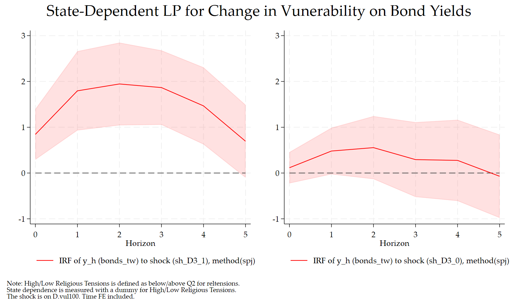
The objective is to test whether the response of sovereign bond yields to a vulnerability shock differs across two regimes of religious tensions. In other words, we want to test whether the coefficient on the shock is statistically different when the regime dummy is equal to one and when the regime dummy is equal to zero.
In the previous locproj blog, this type of test was straightforward because Stata’s test command could be applied directly after each local projection regression. With xtlp, the logic is the same, but the implementation is slightly different because xtlp stores the results horizon by horizon when several horizons are estimated in the same command.
The economic null hypothesis is:
for each horizon .
In the code, the two regime-specific shocks are:
sh_D3_1 = D3   * Dvul100
sh_D3_0 = D3_0 * Dvul100
Thus, the test becomes:
test (_b[sh_D3_1] = _b[sh_D3_0])
This is the xtlp equivalent of the locproj test:
test (_b[0.D3#c.Dvul100] = _b[1.D3#c.Dvul100])
The only difference is that, with xtlp, we have manually created the two interaction terms instead of relying directly on Stata’s factor-variable notation.
Step 1: Create the regime dummy
The first part of the code defines the religious-tensions regime:
cap drop reltensions_p50
cap drop D3
cap drop D3_0
cap egen reltensions_p50 = pctile(reltensions), p(50)gen byte D3 = .
replace D3 = 1 if L.reltensions <  L.reltensions_p50
replace D3 = 0 if L.reltensions >= L.reltensions_p50 ///
    & !missing(L.reltensions, L.reltensions_p50)gen byte D3_0 = 1 - D3 if !missing(D3)
The command:
egen reltensions_p50 = pctile(reltensions), p(50)
computes the median of reltensions. Then, the dummy D3 is defined using the lagged value of religious tensions.
The rule is:
D3 = 1 if L.reltensions < median(reltensions)
D3 = 0 if L.reltensions >= median(reltensions)
So, with this coding, D3=1 corresponds to the below-median religious-tensions regime, while D3=0 corresponds to the above-or-equal-median religious-tensions regime.
This point is important for the interpretation of the figure and the Wald tests. If the variable reltensions is not reverse-coded, then D3=1 is not the high-tension regime; it is the below-median-tension regime.
Step 2: Create the two regime-specific shocks
The two shock variables are then created as:
gen double sh_D3_1 = D3   * Dvul100
gen double sh_D3_0 = D3_0 * Dvul100
These two variables split the same vulnerability shock into two components.
When D3=1:
sh_D3_1 = Dvul100
sh_D3_0 = 0
When D3=0:
sh_D3_1 = 0
sh_D3_0 = Dvul100
So the coefficient on sh_D3_1 measures the response of bond yields to the vulnerability shock in the D3=1 regime, while the coefficient on sh_D3_0 measures the response of bond yields to the same shock in the D3=0 regime.
This is the key idea behind the state-dependent local projection. Instead of estimating one shock coefficient, we estimate two state-specific shock coefficients.
Step 3: Why do we need a helper program?
The helper program is:
cap program drop post_xtlp_h
program define post_xtlp_h, eclass
    args B V
    ereturn post `B' `V'
    ereturn local cmd "post_xtlp_h"
end
This small program is needed because xtlp stores the results differently when we estimate several horizons at once.
After a command like:
xtlp bonds_tw ///
    sh_D3_1 sh_D3_0 ///
    L(1/5).bonds_tw ///
    F(1/5).Dvul100, ///
    tfe method(spj) hor(5) ytransf(level) shock(2) g
xtlp estimates the local projections for horizons 0 to 5. The package documentation indicates that, when multiple horizons are requested, xtlp estimates the model separately for each horizon and stores horizon-specific coefficient vectors and variance-covariance matrices as e(bh) and e(Vh). It also stores a consolidated IRF matrix e(irf).
So after hor(5), the relevant stored matrices are:
e(b0)   e(V0)
e(b1)   e(V1)
e(b2)   e(V2)
e(b3)   e(V3)
e(b4)   e(V4)
e(b5)   e(V5)
where:
e(b0)
is the coefficient vector for horizon 0, and:
e(V0)
is the variance-covariance matrix for horizon 0.
Similarly:
e(b3)
and:
e(V3)
contain the coefficient vector and variance-covariance matrix for horizon 3.
The problem is that Stata’s standard postestimation command:
test
does not automatically know that we want to test coefficients inside e(b0) or e(b3). The command test normally looks for the active coefficient vector e(b) and the active variance-covariance matrix e(V).
The helper program solves this problem. It takes a horizon-specific coefficient vector and variance-covariance matrix and posts them as the active estimation result.
For example:
post_xtlp_h B3 V3
makes Stata behave as if the horizon-3 regression had just been estimated. After that, the command:
test (_b[sh_D3_1] = _b[sh_D3_0])
correctly tests equality of the two state-specific coefficients at horizon 3.
Step 4: Estimate the state-dependent panel local projection
The core xtlp command is:
xtlp bonds_tw ///
    sh_D3_1 sh_D3_0 ///
    L(1/5).bonds_tw ///
    F(1/5).Dvul100, ///
    tfe method(spj) hor(5) ytransf(level) shock(2) g
The dependent variable is:
bonds_tw
The first two regressors are:
sh_D3_1 sh_D3_0
These are the two state-specific shocks.
The option:
shock(2)
tells xtlp that the first two variables in the list of regressors are the shocks for which impulse responses should be reported. This is essential. If we forgot shock(2), xtlp would treat only the first variable as the shock by default. The documentation states that shock(#) treats the first # regressors as separate shocks; for example, shock(2) reports one IRF for the first shock and one IRF for the second shock.
The control variables are:
L(1/5).bonds_tw
F(1/5).Dvul100
The first term includes five lags of bond yields. The second term includes future values of the vulnerability shock as controls.
The option:
tfe
includes two-way fixed effects: individual fixed effects and time fixed effects. In this application, if the panel is declared as:
xtset imfcode period
then tfe corresponds to country fixed effects plus period fixed effects. The xtlp documentation defines tfe as the option that includes both individual and time fixed effects.
The option:
method(spj)
uses the split-panel jackknife estimator. This is one of the main advantages of xtlp: the package provides both the standard fixed-effects estimator, method(fe), and the split-panel jackknife estimator, method(spj). The latter is designed to address the Nickell-type bias that may arise in panel local projections with fixed effects.
Finally:
hor(5)
estimates horizons 0 through 5, and:
ytransf(level)
uses the level of the dependent variable at each horizon. The documentation describes ytransf(level) as using yi,t+h as the dependent variable.
Step 5: Save the horizon-specific results
After running xtlp, the code saves the coefficient and variance-covariance matrices for all horizons:
forvalues v = 0(1)5 {
    matrix B`v' = e(b`v')
    matrix V`v' = e(V`v')
}
This creates:
B0 = e(b0)
V0 = e(V0)
B1 = e(b1)
V1 = e(V1)
...
B5 = e(b5)
V5 = e(V5)
This step is important because once we start posting horizon-specific results using the helper program, the active e() results will be replaced. Therefore, it is safer to copy all matrices first.
Step 6: Run the Wald test horizon by horizon
The final loop is:
forvalues v = 0(1)5 {
    post_xtlp_h B`v' V`v'
    di as text " "
    di as text "Horizon `v'"
    test (_b[sh_D3_1] = _b[sh_D3_0])
}
At each horizon, the command:
post_xtlp_h B`v' V`v'
loads the coefficient vector and variance-covariance matrix for that horizon.
Then:
test (_b[sh_D3_1] = _b[sh_D3_0])
runs a Wald test of equality between the two state-specific coefficients.
The null hypothesis is:
Equivalently:
If the p-value is small, we reject equality and conclude that the vulnerability shock has a statistically different effect across the two regimes at that horizon.
If the p-value is large, we do not reject equality. In that case, the two IRFs may look different visually, but the difference is not statistically significant at that horizon.
The Wald statistic
The test uses the full variance-covariance matrix. This matters because the two estimated coefficients are obtained from the same regression, so they may be correlated.
At horizon , the Wald statistic is:
where:
is the coefficient on sh_D3_1, and:
is the coefficient on sh_D3_0.
The denominator includes the covariance term:
This is why it is better to use Stata’s test command, or the full e(Vh) matrix, rather than comparing the two confidence intervals visually.
Interpretation of the output
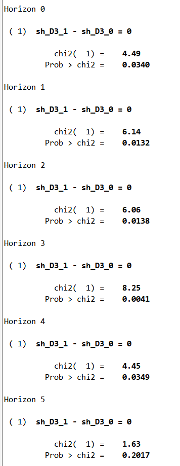
The output has the form:
Horizon 0

 ( 1)  sh_D3_1 - sh_D3_0 = 0
           chi2(  1) =    ...
         Prob > chi2 =    ...
The line:
sh_D3_1 - sh_D3_0 = 0
is exactly the restriction being tested.
The value:
Prob > chi2
is the p-value of the Wald test.
For example, if the output is:
Horizon 0

           chi2(  1) =    4.49
         Prob > chi2 =    0.0340
then the equality of the two regime-specific coefficients is rejected at the 5 percent level at horizon 0.
If instead the output is:
Horizon 5
           chi2(  1) =    1.63
         Prob > chi2 =    0.2017
then the equality of the two regime-specific coefficients is not rejected at horizon 5.
Thus, the test can tell us whether state dependence is present at short horizons, medium horizons, or throughout the full impulse-response path.
Relation with the locproj test
With locproj, the test was:
test (_b[0.D3#c.Dvul100] = _b[1.D3#c.Dvul100])
With xtlp, after manually creating the two shocks, the equivalent test is:
test (_b[sh_D3_1] = _b[sh_D3_0])
The null hypothesis is the same.
The difference is practical. In locproj, one typically estimates one horizon and then runs test immediately. In xtlp, one command estimates the full sequence of horizons, so we must retrieve the horizon-specific coefficient and variance-covariance matrices before applying test.
Therefore, this loop:
forvalues v = 0(1)5 {

    post_xtlp_h B`v' V`v'
    di as text " "
    di as text "Horizon `v'"
    test (_b[sh_D3_1] = _b[sh_D3_0])
}
is the xtlp counterpart of running locproj horizon by horizon and applying test after each regression.
A small warning on exact comparability
The Wald test is aligned with the locproj logic, but the numerical results will be identical only if the estimation specifications are also aligned.
For example, the following option:
method(spj)
uses the split-panel jackknife estimator. This is not the same estimator as the standard fixed-effects estimator used in a command such as:
locproj ..., fe cluster(imfcode)
If the objective is to reproduce the locproj fixed-effects results as closely as possible, use:
method(fe)
If the objective is to report the bias-corrected xtlp results, then:
method(spj)
is appropriate.
The same point applies to the controls. If the locproj specification used one lag of the dependent variable and one lag of the shock, then the xtlp specification should include the corresponding controls. For example:
xtlp bonds_tw ///
    sh_D3_1 sh_D3_0 ///
    L.bonds_tw L.sh_D3_1 L.sh_D3_0 ///
    F(1/5).Dvul100, ///
    tfe method(fe) hor(5) ytransf(level) shock(2) g
would be closer to a locproj specification with:
yl(1) sl(1) c(f(1/5).Dvul100 i.period)
By contrast, the command:
xtlp bonds_tw ///
    sh_D3_1 sh_D3_0 ///
    L(1/5).bonds_tw ///
    F(1/5).Dvul100, ///
    tfe method(spj) hor(5) ytransf(level) shock(2) g
is a valid xtlp specification, but it is not mechanically identical to the original locproj fixed-effects specification.
So the correct interpretation is:
The test is the same state-dependence test as in
locproj, but the numerical results correspond to thextlpspecification that is actually estimated.
Complete code
The full code is:
**# SLP with xtlp

use data_EE.dta, clear
cap drop reltensions_p50
cap drop D3
cap drop D3_0
cap egen reltensions_p50 = pctile(reltensions), p(50)gen byte D3 = .
replace D3 = 1 if L.reltensions <  L.reltensions_p50
replace D3 = 0 if L.reltensions >= L.reltensions_p50 ///
    & !missing(L.reltensions, L.reltensions_p50)

gen byte D3_0 = 1 - D3 if !missing(D3)
label var D3   "D3=1: lagged reltensions below p50"
label var D3_0 "D3=0: lagged reltensions above/equal p50"
cap drop sh_D3_1
cap drop sh_D3_0
gen double sh_D3_1 = D3   * Dvul100
gen double sh_D3_0 = D3_0 * Dvul100
label var sh_D3_1 "D3=1 x D.vul100"
label var sh_D3_0 "D3=0 x D.vul100"

*------------------------------------------------------------
* Helper program: posts one horizon's b and V so that test works
*------------------------------------------------------------

cap program drop post_xtlp_h
program define post_xtlp_h, eclass
    args B V
    ereturn post `B' `V'
    ereturn local cmd "post_xtlp_h"
end

**# Estimate state-dependent LP with xtlp

xtlp bonds_tw ///
    sh_D3_1 sh_D3_0 ///
    L(1/5).bonds_tw ///
    F(1/5).Dvul100, ///
    tfe method(spj) hor(5) ytransf(level) shock(2) g

*------------------------------------------------------------
* Save all horizon-specific coefficient and VCV matrices
*------------------------------------------------------------

forvalues v = 0(1)5 {
    matrix B`v' = e(b`v')
    matrix V`v' = e(V`v')
}

*------------------------------------------------------------
* Wald tests horizon by horizon
* H0: beta(sh_D3_1) = beta(sh_D3_0)
*------------------------------------------------------------

forvalues v = 0(1)5 {
    post_xtlp_h B`v' V`v'
    di as text " "
    di as text "Horizon `v'"
    test (_b[sh_D3_1] = _b[sh_D3_0])
}
Conclusion
This procedure allows us to test whether the effect of a vulnerability shock on bond yields is statistically different across two religious-tensions regimes. The key idea is to split the shock into two regime-specific variables, estimate both IRFs jointly with xtlp, and then test equality of the two coefficients at each horizon.
This is useful because visual differences between impulse responses are not enough. Two IRFs may look different, but the relevant question is whether the difference is statistically significant. The Wald test answers exactly this question.
In the context of state-dependent local projections, this gives a clean way to move from:
“The two IRFs look different”
to:
“The two IRFs are statistically different at horizon h.”
This type of horizon-by-horizon comparison is particularly relevant in applications studying heterogeneous responses to geopolitical, institutional, fiscal, or vulnerability shocks. In the Caldara et al. replication context, the broader empirical motivation is to study how geopolitical and related risks transmit differently across countries, periods, and states, which makes state-dependent LPs and formal equality tests natural tools for the analysis.
References
Saadaoui, J., Beirne, J., Park, D., & Uddin, G. S. (2026). Impact of climate vulnerability on fiscal risk: Do religious tensions and financial development matter? Energy Economics, 109180.
Mei, Z., Sheng, L., & Shi, Z. (2026). Nickell bias in panel local projection: Financial crises are worse than you think. Journal of International Economics, 104210.