I am pleased to announce that I will be contributing blog posts to Timberlake Consultants. The first article, “Geopolitical Shocks and Oil Prices: Local Projections using Stata’s lpirf”, is now available. It uses monthly data to trace the response of real oil prices to geopolitical acts.
This companion post opens up the calculations behind that exercise. Starting from 03_mata.do, we follow the construction of the sample, estimate the local projections through matrix operations in Mata, compute heteroskedasticity-robust standard errors, and return the results to Stata for storage and plotting.
The central part of the post explains Section 3, where QR least squares and the HC0 covariance estimator are implemented, and Section 4, where the resulting matrix becomes a dataset. Each code block below reproduces the corresponding part of the do-file.
Code and data. Download 03_mata.do and November_GPR_Oil_Monthly.dta. Save them in the same folder and make that folder Stata’s working directory before running the complete do-file. The code starts with version 18.0.
The repository folder also contains the companion lpirf and manual-regression versions.
The regression behind the response curve
Let \(y_t\) denote 100 times the logarithm of the real Brent oil price, \(q_t\) the logarithm of world industrial production, and \(g_t\) the geopolitical acts index, gpr_acts. At each horizon \(h=0,\ldots,48\), the do-file estimates
\[ y_{t+h}=\alpha_h+\beta_h g_t +\sum_{\ell=1}^{13}a_{h\ell}q_{t-\ell} +\sum_{\ell=1}^{13}c_{h\ell}y_{t-\ell}+u_{t,h}. \tag{1} \]
The coefficient \(\beta_h\) is the response of interest. The controls absorb the preceding 13 months of global activity and oil prices, with their coefficients estimated separately at every horizon. The code uses 12 baseline lags plus one additional lag. GPRA enters contemporaneously; its own lags and current industrial production are absent from the regressor list.
The shock interpretation follows the short-run exogeneity assumption in the Timberlake article: conditional on the included lag history, contemporaneous economic disturbances do not determine geopolitical acts within the month, while oil prices can respond immediately. The matrix code estimates the coefficient on GPRA directly. Its impulse unit is one GPRA index point; the script applies no standard-deviation rescaling.
Because the dependent variable is \(100\ln(\text{real oil price})\), \(\beta_h\) is measured in log percentage units and approximates a percentage response. The exact percentage conversion for a one-point impulse is \(100[\exp(\beta_h/100)-1]\). Each horizon describes the oil-price level at that date. The curve is formed by placing these coefficients next to one another; the code does not sum them across horizons.
In Stata’s lpirf terminology, coefficients on a contemporaneous exogenous impulse are dynamic multipliers. This is the object reconstructed by the Mata do-file.
Section 1 — Settings and data
version 18.0
clear all
set more off

**# 1. Settings and data

global oil "brent"
global p 12
global H 49
global p_aug = $p + 1
global hmax = $H - 1

capture mkdir "output"
capture log close mata_log
log using "output/03_mata.log", text replace name(mata_log)

use "November_GPR_Oil_Monthly.dta", clear
keep if inrange(month, tm(1985m1), tm(2026m6))
tsset month, monthly
generate double log_oil = 100 * ln_real_${oil}
version 18.0 selects Stata 18 command behavior. clear all initializes the session, and set more off lets output proceed without pagination. The globals define the experiment in one place: Brent is the selected oil series, p_aug evaluates to 13, and hmax evaluates to 48. Thus H = 49 counts the horizons including impact, \(h=0\).
capture mkdir attempts to create the output folder and lets execution continue if it already exists. The next two lines close any log named mata_log and open a fresh text log. replace permits the previous log to be overwritten.
The dataset is restricted to January 1985–June 2026. tsset month, monthly declares the calendar so that Stata’s lag and lead operators refer to months. The expression ln_real_${oil} expands to ln_real_brent. Multiplication by 100 sets the response scale, while double retains double precision in the generated variable.
Section 2 — Regressors, outcomes, and a common sample
2.1 Build the regressor list
generate byte lp_sample = !missing(gpr_acts)
local xvars "gpr_acts"
local yvars ""

forvalues j = 1/$p_aug {
    generate double ip_l`j' = L`j'.ln_world_ip
    generate double oil_l`j' = L`j'.log_oil
    replace lp_sample = 0 if missing(ip_l`j', oil_l`j')
    local xvars "`xvars' ip_l`j' oil_l`j'"
}
lp_sample is a zero–one indicator. It starts at one wherever GPRA is observed. At each lag, the loop creates one industrial-production variable and one oil-price variable. If either is missing, that base date is excluded by setting the indicator to zero.
The local macro xvars collects the names in this exact order:
gpr_acts ip_l1 oil_l1 ip_l2 oil_l2 ... ip_l13 oil_l13There are 27 variables at this point: one impulse and 26 lagged controls. The order matters because the GPRA coefficient will occupy the first row of the coefficient matrix. Mata will append the constant as the final column of the design matrix.
2.2 Build the outcomes at all horizons
forvalues h = 0/$hmax {
    if `h' == 0 {
        generate double oil_f`h' = log_oil
        generate double ip_f`h' = ln_world_ip
    }
    else {
        generate double oil_f`h' = F`h'.log_oil
        generate double ip_f`h' = F`h'.ln_world_ip
    }
    replace lp_sample = 0 if missing(oil_f`h', ip_f`h')
    local yvars "`yvars' oil_f`h'"
}
For \(h=0\), the dependent variable is the current oil price. For \(h>0\), F`h'.log_oil supplies the oil price \(h\) months ahead. The local macro yvars therefore becomes oil_f0 oil_f1 ... oil_f48.
Sample eligibility is checked against every oil-price lead and industrial-production lead. The activity leads enter this selection rule to match the companion lpirf ln_world_ip log_oil exercise. Their role is confined to selecting observations: only oil-price outcomes enter the matrix Y, and all activity regressors in equation (1) are lagged.
This produces one common set of base dates for all 49 regressions. With the supplied data, the 498-month window loses 13 initial base dates to lag construction and 48 final base dates to the longest lead: \(498-13-48=437\). The retained base dates run from February 1986 to June 2022. For the last base date, the 48-month outcome is observed in June 2026.
2.3 Record the sample
count if lp_sample
preserve
keep month lp_sample
save "output/03_sample.dta", replace
restore
count if lp_sample reports 437 in the Stata log. preserve temporarily protects the working dataset while a two-variable file containing month and lp_sample is saved. Because keep month lp_sample selects columns, the saved file retains both included and excluded dates. restore then brings back the variables needed for estimation.
Section 3 — OLS and HC0 in Mata
The next section performs the econometric calculations. One matrix holds the common regressors; another holds the 49 dependent-variable vectors. Reusing the same design matrix makes it possible to calculate all coefficient vectors in one multiplication.
3.1 Define the function and move the data into Mata
mata:
real matrix video_mata_lp()
{
    real matrix X, Y, P, B, U, V, results
    real scalar n, k, rankx, j, bh, seh, z

    X = st_data(., tokens(st_local("xvars")), "lp_sample")
    Y = st_data(., tokens(st_local("yvars")), "lp_sample")
    n = rows(X)
    X = X, J(n, 1, 1)
    k = cols(X)
mata: enters Mata, Stata’s matrix programming language. The declaration real matrix video_mata_lp() defines a function returning a real-valued matrix. The following declarations identify the matrix objects and scalar quantities used inside it.
In st_data(., tokens(st_local("xvars")), "lp_sample"), three operations connect the Stata data to the matrix calculation:
st_local("xvars")reads the text of the Stata local macro.tokens()splits that text into individual variable names.st_data()copies those columns for observations selected bylp_sample. The dot in its first argument makes all observation positions eligible before that selection.
The corresponding expression for yvars creates Y using the same rows. The command J(n, 1, 1) creates a column of \(n\) ones. In X = X, J(n, 1, 1), the comma concatenates that column horizontally with the existing regressors. Hence k = cols(X) returns 28.
Writing one row explicitly makes the column order clear:
\[ x_t’=\bigl(g_t,\ q_{t-1},\ y_{t-1},\ \ldots,\ q_{t-13},\ y_{t-13},\ 1\bigr). \tag{2} \]
For the common base dates \(t_1,\ldots,t_N\), define \(y_h=(y_{t_1+h},\ldots,y_{t_N+h})’\). The full outcome matrix is \(Y=[y_0\;y_1\;\cdots\;y_{48}]\). All rows of \(X\) and \(Y\) refer to the same base dates.
| Object | Dimensions | Contents |
|---|---|---|
X |
437 × 28 | GPRA, 26 lagged controls, and a constant |
Y |
437 × 49 | Oil-price outcomes at horizons 0–48 |
P |
28 × 437 | Operator mapping outcomes into OLS coefficients |
B |
28 × 49 | One coefficient vector per horizon |
U |
437 × 49 | One residual vector per horizon |
V |
28 × 28 | HC0 covariance matrix for the current horizon |
results |
49 × 6 | One output row per horizon |
3.2 Check the sample size and construct the OLS operator
    if (n <= k) {
        errprintf("Too few complete observations.\n")
        _error(2001)
    }

    P = qrsolve(X, I(n), rankx)
    if (rankx < k) {
        errprintf("The design matrix is not full rank.\n")
        _error(459)
    }
The first guard requires more observations than regressors, including the constant. If \(n\leq k\), the function prints a message and stops. After the QR calculation, the second guard requires full numerical column rank. These checks establish the conditions used in the matrix identities below.
The central command is P = qrsolve(X, I(n), rankx). Here I(n) is the \(N\times N\) identity matrix. The call asks Mata to solve the matrix least-squares problem with X as the regressor matrix and the columns of the identity as the right-hand sides. It returns a \(k\times N\) matrix and writes the computed rank into rankx.
Why does that produce the right operator? For one outcome vector, OLS minimizes \((y_h-Xb_h)'(y_h-Xb_h)\). Its first-order condition is \(X’X\widehat b_h=X’y_h\). With full column rank, this gives
\[ \widehat b_h=P y_h, \qquad P=(X’X)^{-1}X’. \tag{3} \]
Applying the same least-squares formula to the identity matrix gives \((X’X)^{-1}X’I_N=P\). This is why I(n) appears in the call. The result is an operator that can subsequently be applied to any of the 49 outcome columns.
The code obtains this operator through QR decomposition. To see the algebra, write a thin QR factorization as \(X=QR\), where \(Q’Q=I_k\) and \(R\) is a nonsingular upper-triangular matrix. Then
\[ \begin{aligned} P&=(R’R)^{-1}R’Q’\\ &=R^{-1}(R’)^{-1}R’Q’\\ &=R^{-1}Q’. \end{aligned} \tag{4} \]
The displayed inverse describes the mathematical solution. The solver uses QR and triangular solves; the code never explicitly forms and inverts \(X’X\). Mata also handles any column permutation used by its QR algorithm internally.
Which product is an identity? The operator satisfies \(PX=I_k\). In the reverse order, \(XP=X(X’X)^{-1}X’\) is the \(N\times N\) projection onto the columns of \(X\). Thus qrsolve(X, I(n), rankx) solves \(XP\approx I_N\) in the least-squares sense. Multiplying \(XP\) by an outcome vector produces its fitted values.
Reading the log. Mata may print “variable rankx may be used before set.” The third argument of qrsolve() is an output argument: the call assigns the rank before the subsequent if statement reads it. In the supplied log, execution continues through estimation, export, and graph creation.
3.3 Calculate all coefficients and residuals
    B = P * Y
    U = Y - X * B
    z = invnormal(0.95)
    results = J(cols(Y), 6, .)
Once P is available, the first two lines implement
\[ \begin{aligned} B&=PY=[\widehat b_0\;\widehat b_1\;\cdots\;\widehat b_{48}],\\ U&=Y-XB=[\widehat u_0\;\widehat u_1\;\cdots\;\widehat u_{48}]. \end{aligned} \tag{5} \]
The same \(P\) operates on every column of \(Y\), so each column of \(B\) equals the OLS estimate from the corresponding horizon regression. The coefficients remain unrestricted across horizons. The first row of \(B\) contains the entire GPRA response curve; the last row contains the intercepts.
U = Y - X * B subtracts fitted values from observed outcomes. Its column \(j\) contains the residuals for horizon \(h=j-1\). These residuals change with the horizon even though the regressor matrix remains fixed.
z = invnormal(0.95) sets the critical value to approximately 1.644854. A central 90% normal interval leaves 5% in each tail, hence the 0.95 quantile. Finally, J(cols(Y), 6, .) allocates a 49-by-6 matrix filled with missing values, ready for the results.
3.4 Form the HC0 covariance matrix
    for (j = 1; j <= cols(Y); j++) {
        // HC0: P * diag(u_h^2) * P', with no N/(N-k) factor.
        V = quadcross(P', U[, j]:^2, P')
        bh = B[1, j]
        seh = sqrt(V[1, 1])
        results[j, .] = (j-1, bh, seh, bh-z*seh, bh+z*seh, n)
    }
The loop visits the 49 columns of Y. At each iteration, U[, j] selects every row of residual column \(j\), and :^2 squares its elements individually. The colon identifies an elementwise operation.
For a given horizon, define \(D_h=\operatorname{diag}(\widehat u_{1,h}^{2},\ldots,\widehat u_{N,h}^{2})\). The HC0 estimator is
\[ \widehat V_h =(X’X)^{-1}X’D_hX(X’X)^{-1} =P D_h P’. \tag{6} \]
The expression in the middle is the familiar sandwich covariance matrix. Substitution of \(P=(X’X)^{-1}X’\) gives the expression on the right. Every observation contributes its own squared residual, allowing its estimated error variance to differ from that of other observations.
The Mata function quadcross(A, w, C) computes \(A’\operatorname{diag}(w)C\). Substituting P' for both A and C therefore yields
\[ \operatorname{quadcross}(P’,\widehat u_h^{\,2},P’) =(P’)’D_hP’=P D_hP’. \tag{7} \]
This explains both transposes in quadcross(P', U[, j]:^2, P'). The function transposes its first argument internally. Passing P' makes that first factor equal to \(P\). The weighted cross-product also avoids constructing the large diagonal matrix \(D_h\) explicitly.
quadcross() accumulates the cross-product sums in quadruple precision and returns a double-precision matrix. The code implements HC0 directly: it applies no \(N/(N-k)\) adjustment. There is also no extra \(1/N\) to append to equation (6), because the scaling is already contained in the two factors of \(P\).
A scalar version gives a useful interpretation. Let \(p_{1i}\) denote entry \(i\) of the first row of \(P\). Then
\[ \widehat\beta_h=\sum_{i=1}^{N}p_{1i}y_{t_i+h}, \qquad \widehat V_{h,11}=\sum_{i=1}^{N}p_{1i}^{2}\widehat u_{i,h}^{2}. \tag{8} \]
The first expression combines the outcomes with the weights relevant to the GPRA coefficient after accounting for the controls. The second expression adds their contributions to its estimated variance. A larger squared residual contributes more, with its influence scaled by the squared coefficient weight. The appendix derives these weights using the Frisch–Waugh–Lovell theorem.
The covariance calculation uses observation-specific squared residuals and the HC0 convention selected in the do-file. Its role here is to construct the pointwise intervals for the specified local projections. The reference to lag-augmented inference follows the framework discussed by Montiel Olea and Plagborg-Møller (2021); the additional lag and the covariance formula are explicit components of this implementation.
3.5 Select the response coefficient and store the interval
bh = B[1, j] selects the GPRA coefficient because GPRA is the first column of X. V[1, 1] is its estimated variance, so sqrt(V[1, 1]) gives its standard error. The stored confidence limits are
\[ \left[\widehat\beta_h-z_{0.95}\,\widehat{\operatorname{se}}(\widehat\beta_h),\quad \widehat\beta_h+z_{0.95}\,\widehat{\operatorname{se}}(\widehat\beta_h)\right]. \tag{9} \]
These are pointwise 90% normal-approximation intervals. The loop computes a within-horizon covariance matrix on each pass; it stores the GPRA standard error and limits needed for the plotted band.
In results[j, .], the dot selects the entire output row. Mata starts indexing at one, whereas the response begins at horizon zero. The expression j-1 therefore creates the correct horizon label.
| Column | Expression | Meaning |
|---|---|---|
| 1 | j-1 |
Horizon, from 0 through 48 |
| 2 | bh |
GPRA response coefficient |
| 3 | seh |
HC0 standard error |
| 4 | bh-z*seh |
Lower pointwise confidence limit |
| 5 | bh+z*seh |
Upper pointwise confidence limit |
| 6 | n |
Common estimation sample size, 437 |
3.6 Return the matrix to Stata
    return(results)
}

st_matrix("LP_result", video_mata_lp())
end
return(results) supplies the function’s output. The call to video_mata_lp() executes the function, and st_matrix() copies its returned matrix into a Stata matrix named LP_result. The final end returns control to Stata. At this point the estimates are available as a 49-by-6 Stata matrix, ready for Section 4.
Section 4 — From a matrix to a results dataset
This section changes the unit of observation. During estimation, a row represents a monthly base date. In the exported dataset, a row represents a projection horizon.
4.1 Name the columns and create variables
matrix colnames LP_result = h b se lb ub N
clear
svmat double LP_result, names(col)
The first line assigns six column names to LP_result: h, b, se, lb, ub, and N. The order matches the six expressions written by the Mata loop.
The following clear removes the current dataset while preserving Stata matrices. Consequently, LP_result remains available. The distinction from the initial clear all matters here: clear all would also erase the results matrix.
svmat double LP_result, names(col) then turns each matrix column into a dataset variable. The option names(col) uses the column names just assigned. The storage type double retains the numerical precision of the estimates and confidence limits. The 49 matrix rows become 49 observations.
Two different observation counts. After svmat, Stata’s _N equals 49, the number of rows in the results dataset. The variable named N equals 437 in every row, recording the number of observations used to estimate each response. The log message resetting the dataset to 49 observations describes this conversion.
4.2 Check the exported structure
sort h
assert _N == $H
assert !missing(b, se, lb, ub)
sort h arranges the records chronologically by horizon. The first assertion requires exactly $H rows, here 49. The second requires a nonmissing coefficient, standard error, and pair of confidence limits in every record. If an assertion fails, Stata stops the do-file. These are checks on the generated output’s structure and completeness.
4.3 Label and save the results
label variable h "Months after the shock"
label variable b "Real oil price response (%)"
label variable se "HC0 standard error"
label variable lb "Lower pointwise 90% confidence limit"
label variable ub "Upper pointwise 90% confidence limit"
label variable N "Common estimation sample size"
save "output/03_mata.dta", replace
export delimited using "output/03_mata.csv", replace
The variable labels make the dataset interpretable when reopened. The saved .dta preserves Stata variable names, storage types, and labels. The CSV provides a portable table of the same numerical columns. Both files use replace, so a new run overwrites earlier outputs with the same names.
For example, the row at h = 12 records an estimated response of approximately 0.03870, an HC0 standard error of 0.01870, and limits of 0.00794 and 0.06946. These fields are sufficient to reproduce the point estimate and its pointwise interval at that horizon.
| h | b | se | lb | ub | N |
|---|---|---|---|---|---|
| 0 | −0.00822 | 0.00561 | −0.01745 | 0.00101 | 437 |
| 2 | −0.01932 | 0.01005 | −0.03585 | −0.00280 | 437 |
| 6 | 0.00005 | 0.01116 | −0.01830 | 0.01840 | 437 |
| 12 | 0.03870 | 0.01870 | 0.00794 | 0.06946 | 437 |
| 24 | 0.06123 | 0.03094 | 0.01034 | 0.11211 | 437 |
| 48 | 0.13115 | 0.03009 | 0.08166 | 0.18065 | 437 |
Coefficients and limits are in log percentage units per one GPRA index point. Entries are rounded to five decimals; the calculations and stored Stata variables use double precision.
Section 5 — Plotting and reading the response
twoway ///
    (rarea lb ub h, fcolor(blue%5) lcolor(blue)) ///
    (line b h, lcolor(red) lwidth(medthick)), ///
    xlabel(0(6)$hmax) ///
    xtitle("Months after the shock") ///
    ytitle("Real oil price response (%)") ///
    title("Real oil price response to a GPR act shock") ///
    subtitle("Pink Sheet series: ${oil}") ///
    note("Unit GPR innovation; pointwise 90% confidence interval.") ///
    legend(off) graphregion(color(white)) ///
    yline(0, lpattern(dash) lcolor(gs10)) ///
    xsize(5) name(GPR_oil_3, replace)

graph export "output/03_mata.png", width(2000) replace
graph save "output/03_mata.gph", replace
log close mata_log
The first plot layer, rarea lb ub h, shades the region between the two confidence limits. fcolor(blue%5) applies a pale blue fill and lcolor(blue) draws its boundary. The second layer, line b h, draws the estimated response in red. The band is drawn first so the response line remains visible above it.
xlabel(0(6)$hmax) labels the horizontal axis every six months through month 48. The axis titles state the horizon and response scale; the title, subtitle, and note identify the impulse, oil series, and interval. legend(off) removes the legend, graphregion(color(white)) sets the background, and yline(0, ...) supplies the dashed zero reference. xsize(5) sets the graph width in inches, and name(..., replace) names the graph in memory.
The figure is exported as a 2,000-pixel-wide PNG and saved as an editable Stata .gph file. The final line closes the named log.
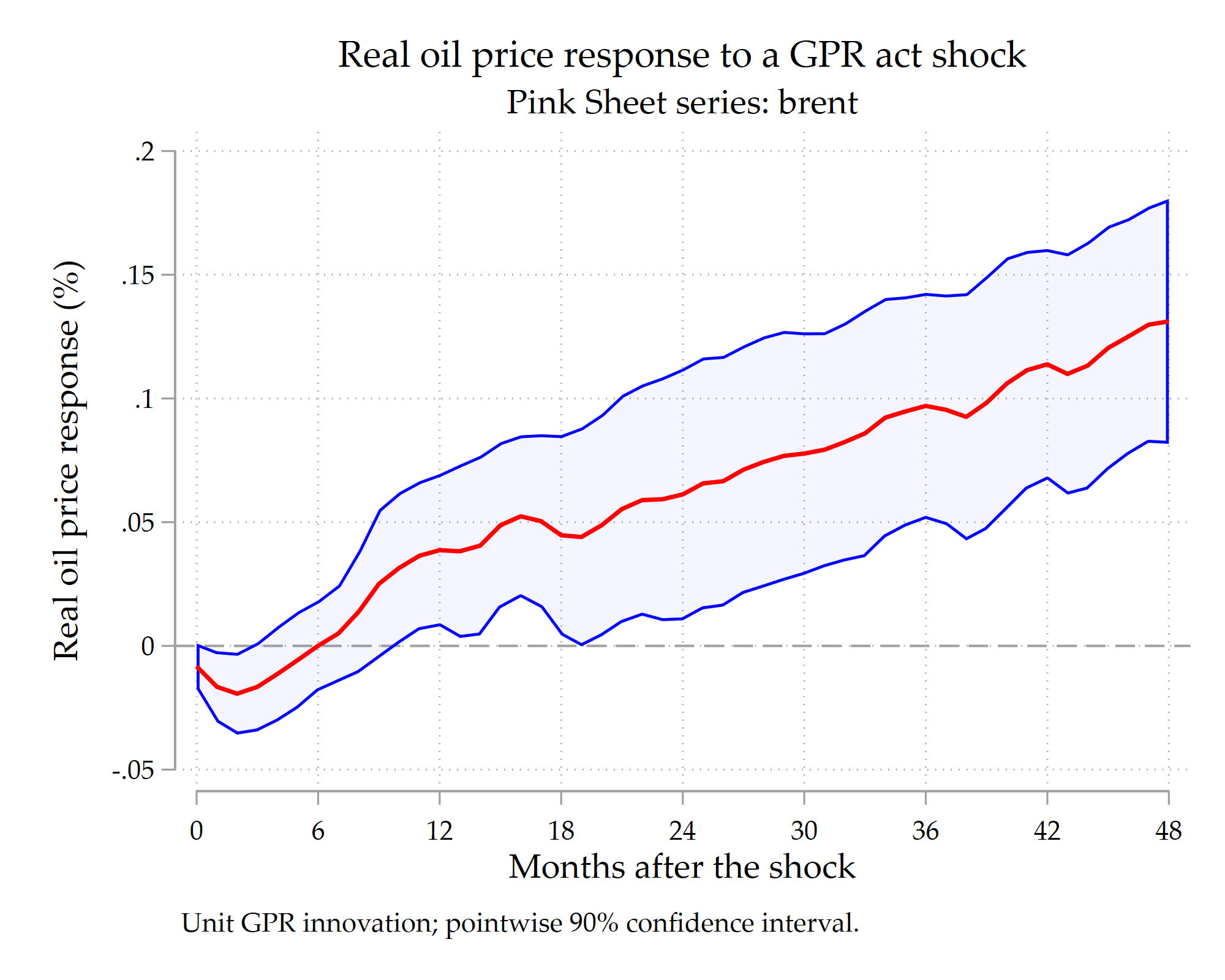
03_mata.do. The red line reports the dynamic multiplier; the shaded region shows pointwise 90% HC0 confidence intervals. The common estimation sample contains 437 monthly base dates. Open the full-size figure.
The response is initially negative, reaching approximately −0.0193% at month two, and is close to zero at month six. It becomes positive thereafter: approximately 0.0387% after 12 months, 0.0612% after 24 months, and 0.1312% after 48 months for a one-point GPRA impulse. At month 48, the pointwise interval runs from about 0.0817% to 0.1806%.
Geopolitical acts can affect oil prices through both global demand and concerns about energy supply. The estimated curve traces the net price response over time. Its change in sign makes the horizon dimension economically meaningful: the immediate movement and the later adjustment convey different parts of the response.
The Mata implementation exposes how that curve is assembled. The common design matrix determines the OLS operator; each outcome column supplies a horizon-specific coefficient vector; each residual column supplies its HC0 covariance; and the exported dataset preserves the coefficient, uncertainty, and sample size needed to draw the figure.
Mathematical appendix — The weights behind the GPRA coefficient
Equation (8) expresses the GPRA coefficient as a weighted sum of outcomes. The Frisch–Waugh–Lovell theorem identifies those weights explicitly.
Partition the design matrix as \(X=[g\;Z]\), where \(g\) is the GPRA column and \(Z\) contains the 26 lagged controls and the constant. Define the residual-maker matrix and residualized GPRA as
\[ M_Z=I_N-Z(Z’Z)^{-1}Z’, \qquad \widetilde g=M_Zg. \tag{10} \]
The full-rank condition checked in Section 3 ensures that the controls are linearly independent and that \(g’M_Zg>0\). Residualizing GPRA removes its linear projection on those controls. This isolates the GPRA variation used to estimate its conditional response coefficient.
The coefficient can be written as
\[ \widehat\beta_h =\frac{g’M_Zy_h}{g’M_Zg} =\frac{\widetilde g’y_h}{\widetilde g’\widetilde g} =\sum_{i=1}^{N} \frac{\widetilde g_i}{\sum_{r=1}^{N}\widetilde g_r^2} \,y_{t_i+h}. \tag{11} \]
The middle equality follows from the symmetry and idempotence of \(M_Z\). Since \(M_Z’=M_Z\) and \(M_Z^2=M_Z\), we have \(\widetilde g’\widetilde g=g’M_Zg\). The corresponding numerator is \(\widetilde g’y_h=g’M_Zy_h\). The outcomes can therefore appear directly in the final weighted sum because the weights already remove the component explained by \(Z\).
Comparing equation (11) with the first row of \(\widehat b_h=Py_h\) gives
\[ p_{1i}=\frac{\widetilde g_i}{\sum_{r=1}^{N}\widetilde g_r^2}, \qquad \widehat{\operatorname{Var}}_{\mathrm{HC0}}(\widehat\beta_h) =\frac{\sum_{i=1}^{N}\widetilde g_i^2\widehat u_{i,h}^{2}} {\left(\sum_{i=1}^{N}\widetilde g_i^2\right)^2}. \tag{12} \]
The residuals \(\widehat u_{i,h}\) in this expression are those of the full horizon regression, exactly as stored in U. The denominator measures GPRA variation remaining after controlling for lagged activity and oil prices. The numerator combines that residualized variation with horizon-specific squared errors. This is the scalar calculation contained in V[1, 1].
Because the sample and controls are common across horizons, the weights \(p_{1i}\) remain fixed. Future oil-price outcomes and regression residuals change with \(h\), producing the changing response curve and confidence-band width.
Sources and documentation
Saadaoui, J. (2026). Geopolitical Shocks and Oil Prices: Local Projections using Stata’s lpirf. Timberlake Consultants, 5 November.
Saadaoui, J. (2026). 03_mata.do and monthly data. Timberlake-blogs, November_2026_Video. Code consulted on 7 November 2026.
Montiel Olea, J. L., and Plagborg-Møller, M. (2021). Local Projection Inference Is Simpler and More Robust Than You Think. Econometrica, 89(4), 1789–1823.
StataCorp. [TS] lpirf: local-projection impulse–response functions and dynamic multipliers.
StataCorp. Mata Reference Manual: st_data(), qrsolve(), quadcross(), and st_matrix().
StataCorp. [D] clear and [P] matrix mkmat / svmat.