What does the tvpreg Stata command do?

A common misunderstanding when first encountering the tvpreg Stata command is to think that it estimates time variation the way a rolling regression does, or the way a kernel-smoothed varying-coefficient model does. That is not what tvpreg does.

This distinction matters because the logic of the estimator is different from both of those familiar approaches. A rolling regression generates time variation by repeatedly re-estimating the model on overlapping subsamples. A kernel-smoothed approach also relies on local estimation, but it gives more weight to observations that are close to a given date and less weight to distant observations, with the bandwidth controlling how local the smoothing is. In both cases, time variation is built from a sequence of local regressions.

The tvpreg command works differently. It does not estimate one regression for each date. It does not use a rolling window. It does not require a kernel or a bandwidth. Instead, it treats the coefficient as a parameter path over the entire sample and estimates that path jointly in an unstable environment.

This is the key idea inherited from the parameter-path framework of Müller and Petalas and extended by Inoue, Rossi, and Wang to local projections, and by Inoue, Rossi, Wang, and Zhou to the Stata implementation in tvpreg. The object of interest is not a collection of local coefficient estimates. The object of interest is the full coefficient path itself.

To see the difference clearly, it helps to start from the constant-parameter benchmark. Suppose that the data are first summarized by a standard constant-parameter model. The relevant question is then not, “What coefficient do I get if I estimate the model again around date $t$?” The relevant question is instead, “If the coefficient is allowed to evolve over time, what full-sample path is most consistent with the information in the data?” That change in perspective is fundamental. The coefficient is treated as one full-sample object, not as a sequence of unrelated local estimates.

A useful summary is the following. tvpreg does not:

• choose a rolling window,
• choose a kernel bandwidth,
• estimate a separate regression at each date,
• select one exact degree of instability and discard all others.

Instead, tvpreg does:

• treat the coefficient as a full-sample path,
• construct candidate paths for different admissible degrees of instability,
• evaluate those candidate paths using a score-Hessian pseudo model,
• combine them through a weighted-average-risk logic.

That last point is central. The C grid in tvpreg is not a bandwidth. It does not tell the command how many nearby observations to use around each date. It does not determine the width of a local neighborhood. Rather, the grid determines how much instability the estimator is allowed to consider when constructing candidate parameter paths.

Small values of C correspond to paths that remain close to the constant-parameter benchmark. Larger values allow the coefficient path to move more over time. So the C grid should be understood as a menu of admissible instability scenarios, not as a smoothing parameter in the usual nonparametric sense.

For example, suppose the grid is $0, 3, 6, 9, 12, 15$. Then tvpreg constructs one candidate coefficient path for each of those values. The path associated with $C = 0$ is essentially the stable benchmark. The path associated with $C = 3$ allows mild instability. The paths associated with $C = 9$ or $C = 15$ allow much more movement over time. So the estimator is not hard-coding one specific form of instability in advance. It is entertaining a range of plausible instability magnitudes and constructing one path for each of them.

This is where the weighted-average-risk logic becomes crucial.

Because the true coefficient path is unobserved, one cannot directly compare an estimated path with the true path in realized data. The problem is not that the method lacks a target. The target is the entire parameter path. The problem is that the target is unknown. For that reason, the estimator is evaluated in terms of expected path-estimation loss over a class of plausible unstable environments, not in terms of a realized comparison with an observed true path.

This is the sense in which the method is rooted in weighted average risk. The estimator is designed to perform well, on average, across a weighted class of admissible instability patterns. It does not assume that the researcher knows in advance exactly how unstable the environment is. It does not pick one value of $C$ once and for all and then proceed as if that value were known to be correct. Instead, it constructs a candidate path for each value in the grid, evaluates how well each candidate is supported by the data, and then combines them.

So the final tvpreg estimate is not “the path for one selected grid value.” It is the weighted average of the candidate paths generated across the grid. In practical terms, the grid supplies the admissible instability scenarios, and the weighting scheme determines how much each scenario contributes to the final estimated path.

This point is worth emphasizing because it is easy to miss. Many users implicitly think in terms of model selection: choose one value, estimate one model, and report one path. But the logic here is closer to model averaging over instability scenarios. Each value of C defines one admissible degree of instability, and the final estimator aggregates across those possibilities rather than committing to one of them ex ante.

The performance criterion is also important. The candidate paths are not evaluated by forecast accuracy. The criterion is not out-of-sample prediction performance, and it is not regression residual variance in the usual sense. The relevant object is the quality of the estimated parameter path itself. More precisely, tvpreg evaluates candidate paths through a pseudo time-varying parameter representation built from the score and Hessian of the constant-parameter model. That pseudo representation delivers a quasi log-likelihood criterion for each candidate path. Better-supported paths receive larger weights, and the final coefficient path is the weighted average across those candidates.

A useful intuition is the following. The score tells us how the data, observation by observation, push the coefficients away from the constant-parameter benchmark. The Hessian provides the local curvature information needed to scale and organize those pushes. The score-Hessian pseudo model then translates this information into candidate time-varying paths and into a criterion for weighting them. So the method uses the constant-parameter model as a starting point, but not as the final answer. It uses that benchmark to construct an approximate full-sample representation of instability.

This is why the smoothness of the tvpreg estimate should not be confused with kernel smoothing. The estimated path is smooth, but the source of that smoothness is the recursion and the persistence structure embedded in the path-estimation problem. The smoothness does not come from fitting local regressions with distance-based weights. It comes from the dynamic construction of admissible parameter paths and from the averaging of those paths under the weighted-average-risk criterion.

With that conceptual background in place, it is useful to look at an empirical application. I use the tvpreg help-file example for the IV-TVP-LP estimator:

///// Estimator III: TVP-LP-IV /////
// Fiscal multiplier
mata: cB = (3*(0::5))'; cB = cB # J(1,6,1)
mata: cv = (3*(0::5))'; cv = J(1,6,1) # cv
mata: cmat = (J(28,1,1) # cB) \ (J(3,1,1) # cv)
mata: st_matrix("cmat",cmat)
tvpreg gdp gs_l* gdp_l* shock_l* (gs = shock), cmatrix(cmat) nwlag(8) nhor(4/20) cum
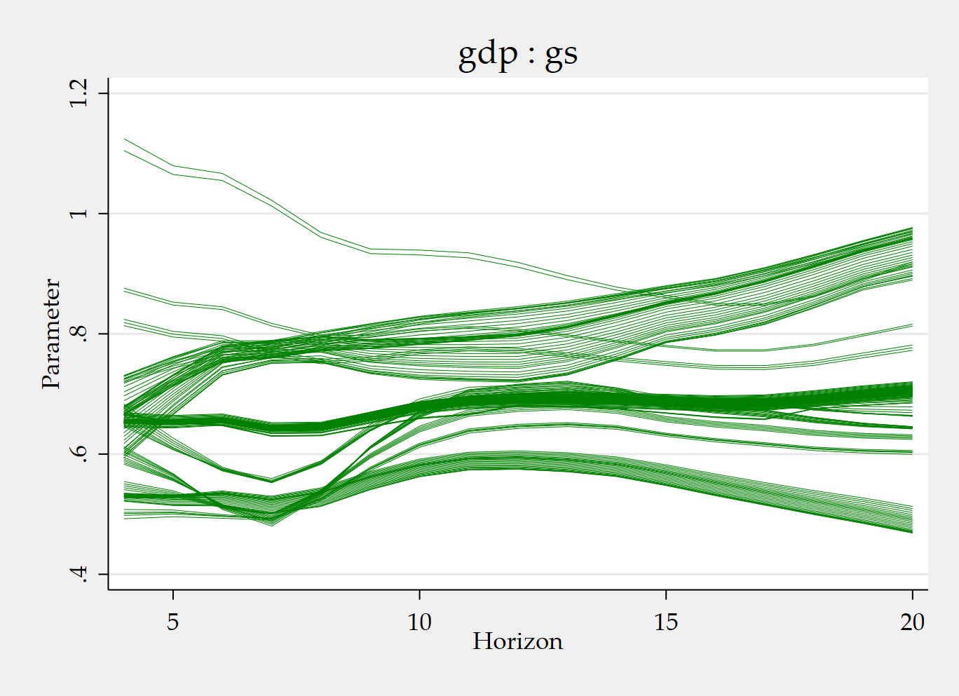
tvpplot, plotcoef(gdp:gs) period(recession) name(figure3_1)
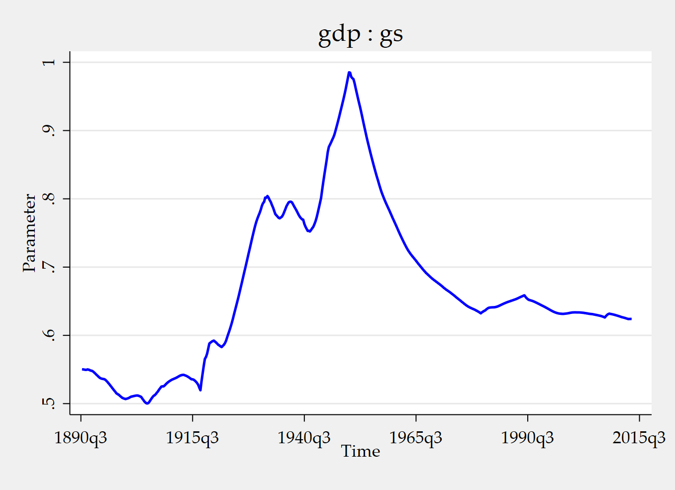
tvpplot, plotcoef(gdp:gs) plotnhor(8) name(figure3_2) 

This example estimates a time-varying IV local-projection specification for the cumulative fiscal multiplier. In this setup, gs is the endogenous regressor, gdp is the dependent variable, and shock is the excluded instrument. The included instruments are the lagged values of gs, gdp, and shock, together with the constant.

The two figures answer two different questions. The first figure shows how the instrumented cumulative fiscal multiplier evolves over time during recession periods. The second figure fixes the horizon at 8 quarters and shows the corresponding time-varying cumulative fiscal multiplier at that horizon. So one figure emphasizes time variation conditional on recession episodes, while the other emphasizes the time-varying response at a particular horizon.

Let me now explain the Mata part, because that is where many users first wonder what the C grid is really doing.

Start with:

mata: cB = (3*(0::5))'; cB = cB # J(1,6,1)

The expression 0::5 generates the sequence $0, 1, 2, 3, 4, 5$. Multiplying by 3 gives the grid $0, 3, 6, 9, 12, 15$. The transpose turns this sequence into a column vector. Then cB # J(1,6,1) replicates that grid across 6 columns. So this line defines the instability grid for the slope block of the parameter vector.

Intuitively, the estimator will consider candidate slope paths associated with different admissible degrees of instability, ranging here from no instability to relatively pronounced instability.

Now consider:

mata: cv = (3*(0::5))'; cv = J(1,6,1) # cv

This does the same thing for the covariance block of the parameter vector. The grid is again $0, 3, 6, 9, 12, 15$, but it is arranged in the way needed for the covariance parameters. So cB controls the instability grid for the slope parameters, while cv controls the instability grid for the covariance parameters.

Then we have:

mata: cmat = (J(28,1,1) # cB) \ (J(3,1,1) # cv)

This is the line that assembles the full C-grid matrix used by tvpreg. It says: repeat the slope grid cB for 28 parameters, then stack underneath it the covariance grid cv for 3 parameters. The result is a block-specific grid for the full parameter vector.

Why 28 slope parameters and 3 covariance parameters in this example?

The answer comes from the dimension of the stacked IV system. In this strong-instrument TVP-IV setup, we have:

• 1 endogenous regressor: gs,
• 1 dependent variable: gdp,
• 1 excluded instrument: shock,
• included instruments given by 4 lags of gs, 4 lags of gdp, 4 lags of shock, plus the constant.

So the number of included instruments is:

$$4 + 4 + 4 + 1 = 13.$$

In the strong-instrument formulation used in the paper, the stacked system has 2 equations: one structural equation and one reduced-form first-stage equation. Each equation has the same 13 included instruments, and the structural equation also contains the contemporaneous endogenous regressor. That gives:

$$13 + 1 = 14$$

slope coefficients per equation block. Since there are 2 equations in the stacked system, the total number of slope parameters is:

$$2 \times 14 = 28.$$

That is the origin of the J(28,1,1) term.

Now turn to the covariance block. Because the stacked system has dimension 2, the covariance matrix is $2 \times 2$. A symmetric $2 \times 2$ covariance matrix has:

$$\frac{2(2+1)}{2} = 3$$

distinct elements. That is the origin of the J(3,1,1) term.

Finally,

mata: st_matrix("cmat",cmat)

transfers the Mata object cmat into Stata as a standard matrix named cmat, so that tvpreg can use it.

This block-specific construction is useful because the full parameter vector generally contains different types of objects. In many applications, one block contains slope coefficients and another block contains covariance parameters. There is no reason to assume that these blocks should be allowed to vary over time in exactly the same way. That is why cB and cv are defined separately.

If you use the same grid for both blocks, you are allowing roughly the same degree of admissible instability in slopes and covariance terms. If you choose a wider grid for cB than for cv, you are allowing slope coefficients to vary more than covariance parameters. So changing cB and cv is not analogous to changing a smoothing bandwidth. It changes the menu of admissible instability magnitudes over which candidate paths are constructed and averaged.

For example, a narrower grid such as $0, 2, 4, 6, 8, 10$ restricts the estimator to relatively mild instability. A wider grid such as $0, 4, 8, 12, 16, 20$ allows stronger movement in the parameter path. The key point is always the same: the grid governs which instability scenarios are admissible, and the final estimate aggregates across those scenarios through the weighted-average-risk logic.

The practical takeaway is straightforward. tvpreg estimates one full-sample coefficient path for each horizon. It does not obtain time variation by repeatedly re-estimating local regressions. The C grid governs how flexible that path is allowed to be. Each value in the grid generates one candidate path. The final estimate is the weighted average of those candidate paths.

So when you choose cB and cv, you are deciding which instability scenarios the estimator is allowed to consider for the slope and covariance blocks. That is the key to understanding what tvpreg does and why the C grid is central to the approach.

References

Inoue, A., Rossi, B., & Wang, Y. (2024). Local projections in unstable environments. Journal of Econometrics, 244(2), 105726.

Inoue, A., Rossi, B., Wang, Y., & Zhou, L. (2025). Parameter path estimation in unstable environments: The tvpreg command. The Stata Journal, 25(2), 374-406.

Ginn, W., Saadaoui, J., & Salachas, E. (2025). Stock Price Bubbles, Inflation and Monetary Surprises. Inflation and Monetary Surprises (September 21, 2025).

Müller, U. K., & Petalas, P. E. (2010). Efficient estimation of the parameter path in unstable time series models. The Review of Economic Studies, 77(4), 1508-1539.

Appendix: How tvpreg constructs the WAR path estimator

The tvpreg command implements a weighted-average-risk (WAR) path estimator in unstable environments. The starting point is a model with time-varying parameters, where the goal is not to estimate one fixed coefficient vector, but the entire parameter path $\{\theta_t\}_{t=1}^T$. The theoretical justification comes from the Müller–Petalas path-estimation framework, and the tvpreg implementation uses a quadratic approximation to the log-likelihood together with a pseudo model based on the score and Hessian.

Formally, tvpreg does not minimize the infeasible realized loss relative to the unknown true path directly. Instead, it computes a family of candidate paths indexed by different instability values $c_i$​, assigns a weight to each candidate using a quasi log-likelihood criterion, and then averages the candidate paths using those weights. In the command’s step-by-step implementation, this is done in 4 main steps.

Step 1. Construct the score-based objects

The first step is to summarize the sample information about the time-varying parameter path using the score and Hessian evaluated at the constant-parameter estimator $\hat\theta$. In the tvpreg notation, one defines for each date $t$ the vectors $e_{x,t}$and $e_{y,t}$ as the elements of $\hat H^{-1}s_t(\hat\theta)$ and $\hat H \hat V^{-1}s_t(\hat\theta)$, respectively. These objects are the building blocks for the pseudo model and contain the relevant local information about parameter instability.

The important point is that the algorithm does not start by estimating a separate regression at each date. Instead, it first extracts from the full sample the score-Hessian objects that summarize how the data push the coefficients away from the constant-parameter benchmark. This is why the procedure is fundamentally different from rolling estimation or kernel smoothing.

Step 2. For each instability value $c_i$, construct one candidate parameter path

This is the key step. For each value $c_i$​ in the user-specified grid

$$C=\{c_0,c_1,\dots,c_{n_G}\}, \qquad c_0=0,$$

the method constructs one candidate path $\{\hat\theta_{i,t}\}_{t=1}^T$​. The first ingredient is the persistence parameter

$$r_i = 1-\frac{c_i}{T}.$$

This parameter determines how persistent the candidate path is. When $c_i$ is small, $r_i$ is close to $1$, so the path is very smooth and close to the stable benchmark. When $c_i$​ is larger, $r_i$​ is smaller, so the path is allowed to adjust more quickly over time. Thus, each $c_i$​ represents one admissible degree of instability.

The algorithm then applies a forward recursion:

$$\zeta_{i,1}=e_{x,1}, \qquad \zeta_{i,t}=r_i\zeta_{i,t-1}+e_{x,t}-e_{x,t-1}, \quad t=2,\dots,T.$$

This recursion accumulates information over time. The term $r_i\zeta_{i,t-1}$ carries past information forward with persistence $r_i$​, while the increment $e_{x,t}-e_{x,t-1}$​ injects the new information coming from date $t$. The variable $\zeta_{i,t}$ is not yet the coefficient path itself; it is an auxiliary state variable that stores the evolving score information under the instability scenario indexed by $c_i$​.

Next, the method residualizes the forward-recursion sequence. Specifically, it regresses the sequence $\{\zeta_{i,t}\}_{t=1}^T$​ on $\{r_i^{\,t-1}I_q\}_{t=1}^T$ and keeps the residuals $\{\zeta^e_{i,t}\}_{t=1}^T$. This step removes the deterministic component associated with the initialization and recenters the recursion so that the subsequent smoothing step focuses on the relevant time variation rather than on an arbitrary starting level.

The algorithm then performs a backward recursion:

$$\zeta_{i,T}=\zeta^e_{i,T}, \qquad \zeta_{i,t}=r_i\zeta_{i,t+1}+\zeta^e_{i,t}-\zeta^e_{i,t+1}, \quad t=1,\dots,T-1.$$

This is the smoothing step. The forward recursion uses information moving from the beginning of the sample to the end, whereas the backward recursion uses information from the end of the sample back to the beginning. After the 2 passes, $\zeta_{i,t}$ becomes a full-sample smoothed object: it reflects not only past information but also future information. This is why the resulting path is smooth without being a kernel-smoothed estimate. The smoothness comes from the dynamic recursion and the persistence parameter $r_i$​, not from local kernel weights or bandwidth choice.

Finally, the candidate parameter path for instability level $c_i$ is obtained as

$$\hat\theta_{i,t}=\hat\theta + e_{x,t} – r_i\zeta_{i,t}, \qquad t=1,\dots,T.$$

This expression shows how the candidate path is built. It starts from the constant-parameter estimate $\hat\theta$, adds a date-specific correction $e_{x,t}$​, and subtracts the smoothed persistence term $r_i\zeta_{i,t}$​. The result is one complete time path of coefficients associated with one particular degree of instability. Repeating this step for all values in the grid $C$ produces a collection of candidate paths.

A useful way to summarize Step 2 is the following: for each $c_i$, tvpreg takes the noisy local score information, propagates it forward through the sample, recenters it, smooths it backward, and turns it into one admissible coefficient path. The role of $c_i$ is to determine how persistent and how variable that candidate path is allowed to be.

Step 3. Convert the candidate paths into weights

Once the candidate paths $\{\hat\theta_{i,t}\}$ have been computed, the algorithm evaluates each instability scenario using a quasi log-likelihood criterion. For each $c_i$​, the command computes $qLL(c_i)$ and an associated unnormalized weight $we_i$. These weights depend on both the persistence parameter $r_i$​ and the quasi log-likelihood contribution of the candidate path. The weights are then normalized as

$$w_i=\frac{we_i}{\sum_{j=0}^{n_G} we_j}.$$

The normalized weights add up to 1 and determine how much influence each candidate path has in the final estimator. Better-supported instability scenarios receive larger weights.

The main conceptual point is that the method does not pick one “best” value of $c_i$​ and discard the others. Instead, it lets the data determine how much weight to place on each admissible instability scenario. This is the practical meaning of the weighted-average-risk logic in the command.

Step 4. Average the candidate paths

The final parameter path estimator is the weighted average of all candidate paths:

$$\hat\theta_t=\sum_{i=0}^{n_G} w_i \hat\theta_{i,t}, \qquad t=1,\dots,T.$$

So the estimated path reported by tvpreg is not the outcome under a single chosen instability level. It is the weighted combination of all the candidate paths in the grid. This is why the estimator is best understood as a model-averaging path estimator over alternative degrees of instability.

In short, the 4-step logic is: first summarize the sample information with score-Hessian objects; second, for each instability value $c_i$, construct one candidate path through forward and backward recursions; third, evaluate each candidate path and compute its weight; and fourth, average all candidate paths using those weights. The estimator is therefore smooth, full-sample, and robust to uncertainty about the exact degree of parameter instability.

The recursion produces a smoothed coefficient path, but this is not kernel smoothing. The smoothness comes from the persistence structure imposed on the latent parameter path through the forward-backward recursion, not from locally weighted regressions based on a kernel and bandwidth.