A few days ago, I assisted to wonderful presentation by Di Liu of StataCorp LLC. His explanations were crystal clear about the difference-in-difference commands introduced in Stata 18. I would like to thank him, Enrique Pinzon and Meghan Cain for their excellent answers to the online participants’ questions. You can find the current list of Stata webinars on the Stata website: https://www.stata.com/.
In this post, I will try to comment his slides in order to give an intuitive understanding of the new commands in Stata 18 that deal with cases of Heterogeneous Difference-in-Differences.
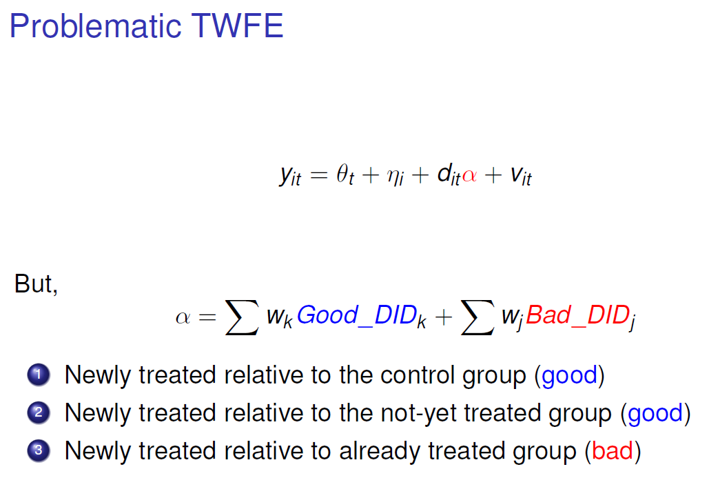
With dit, a dummy variable that indicate the individual i receive the treatment at time t. The first step is to recall that when we use the use the Two Way Fixed Effect (TWFE) estimator, described above, we conflate good comparisons (case 1 and 2) and bad comparisons (case 3). Why? Because, comparing the newly treated group with the control group (case 1) and the not yet treated group (case 2) is valid, since it allows us to identify the effect of the treatment. However, comparing the newly treated group and the already treated group (case 3) is not valid when the effect of the treatment is heterogeneous.
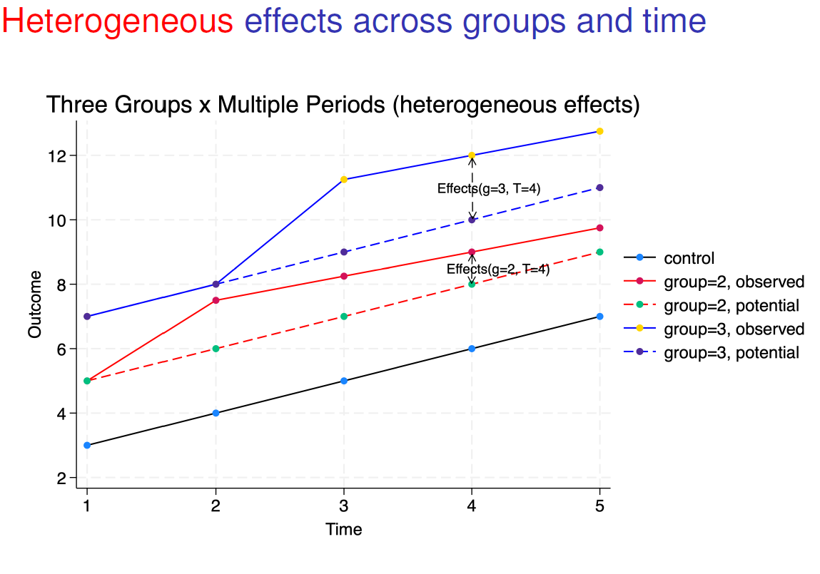
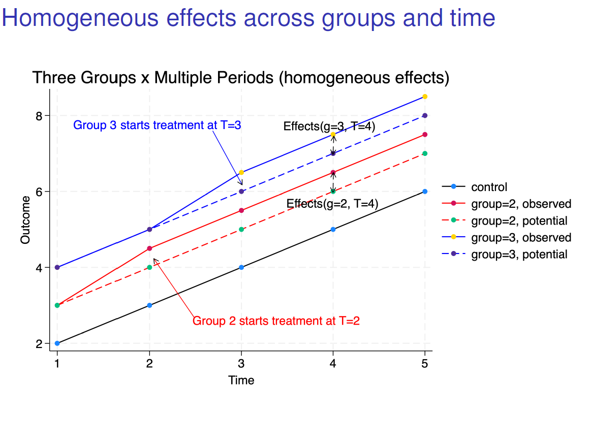
The TWFE estimator is a weighted average of valid comparisons and invalid comparisons in case of heterogeneous effects, because it breaks the parallel trend assumption (plain blue curve against the plain red curve) in the above graphs. In case of homogeneous effect, see below, the TFWE estimator is valid as the parallel trend assumption holds and you can have the average effect on the treated group 3 by comparing the plain blue curve and the plain red curve from the start of the treatment at period T = 3 (recall that it was not the case with heterogeneous effects, the two curves were not parallel anymore).
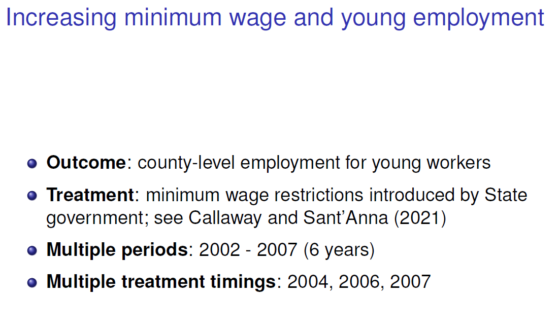
The new Stata 18 commands xthdidregress and hdidregress for panel data and repeated cross-section data estimates four estimators: ra, ipw, aipw in Callaway and Sant’Anna (2021) and twfe in Wooldridge (2021). In order to illustrate the post-estimation commands, I present the following example:
The syntax of the command is especially simply and intuitive:
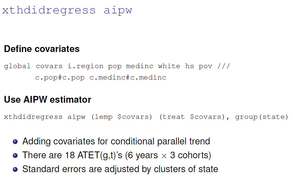
We obtain that the Average Treatment Effect on the Treated (ATET) group:
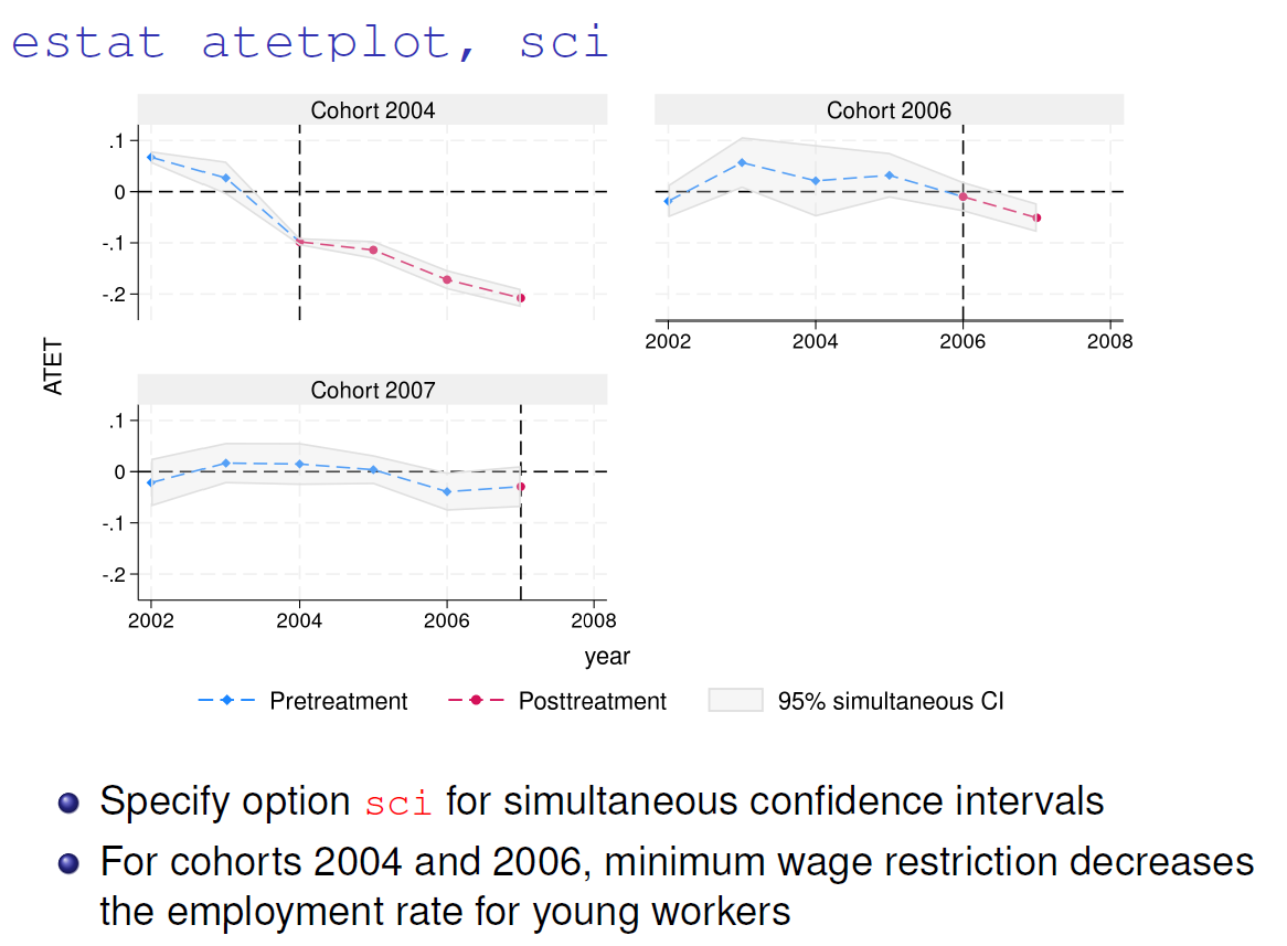
Stata 18 proposes to aggregate the ATET using weighting scheme to have a better visualization. For example, we can answer to the following question:
How do the ATETs vary with the length of exposure to the
treatment? (event study)
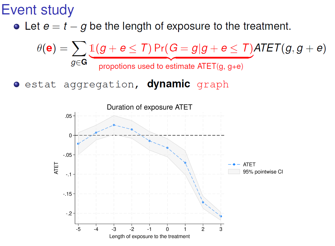
In the figure above g is the starting date for the treatment and e is the duration of exposure to the treatment. In order to give intuition, we can discuss the value in t+3. In our example, the cohort that has been exposed to the treatment during 3 period is the 2004 cohort, the value -0.2 is the value for the 2004 cohort as there is no other value to weight.
We can also try to answer to the following question:
How do the ATETs vary with cohorts? (does start treatment earlier
matter?)
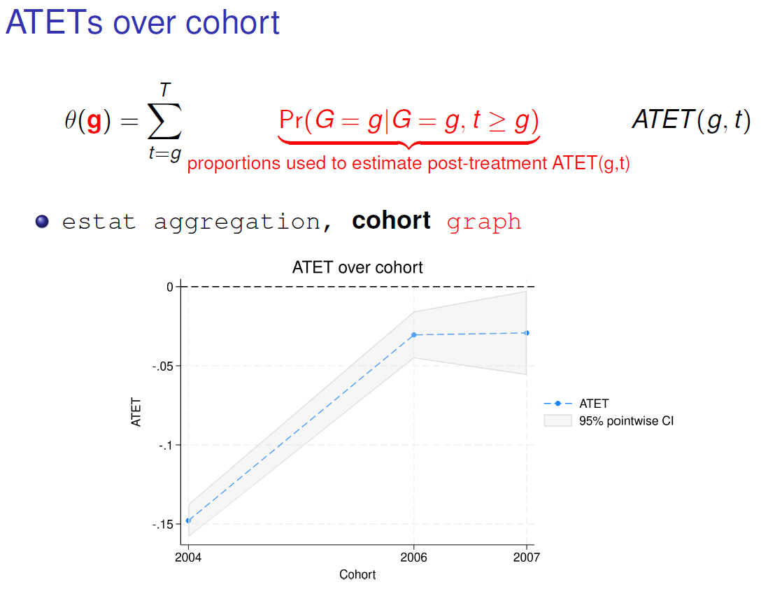
Here, we can observe that the effect in 2004 is -0.15. This value is average of the effects for the cohort 2004 after the start of the treatment. We have four values that fluctuates between -0.1 and -0.2, this we can see how we get -0.15.
We can also try to answer to the following question:
How do the ATETs vary with time? (Good year vs. lousy year)
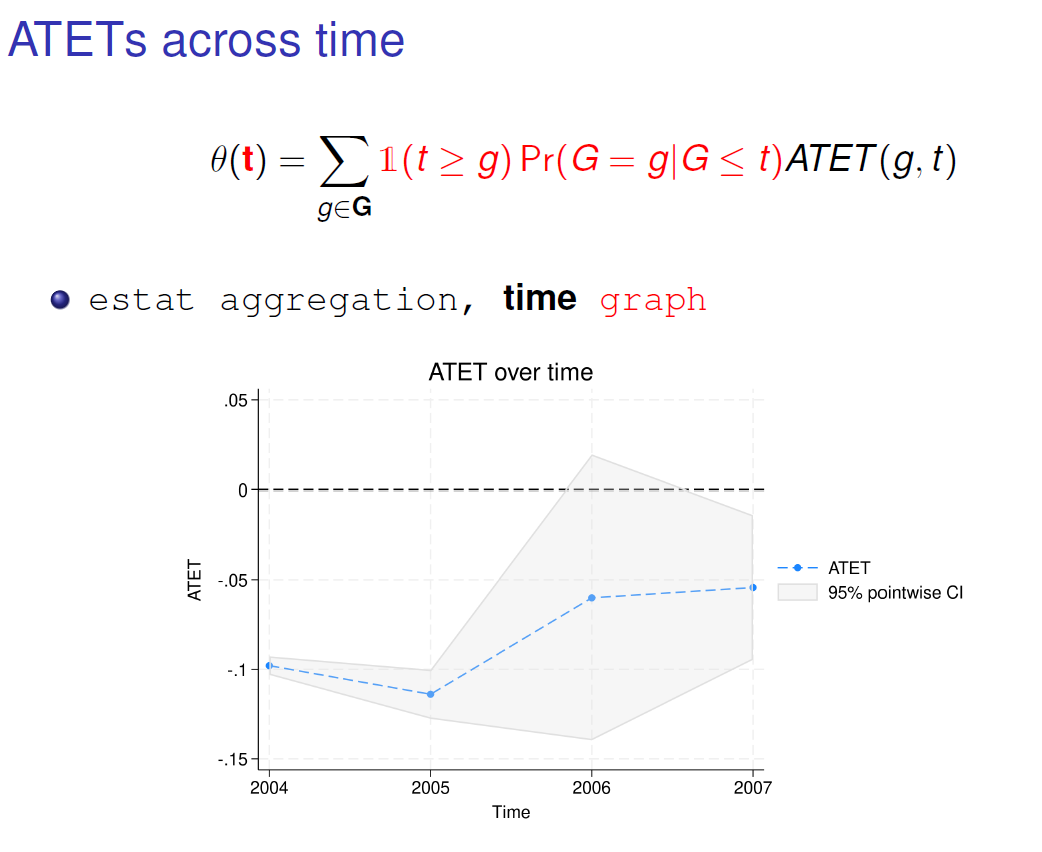
Here, we can observe that the value in 2004 is the same for the 2004 cohort. Why? Because, in 2004, the only treated group was the 2004 cohort thus there is no other value to weight.
Finally, I briefly present the estimators introduce in Stata 18. But, wait, what’s do you really estimate when you run these commands? Let come back to the canonical DID example, with two groups and two periods:
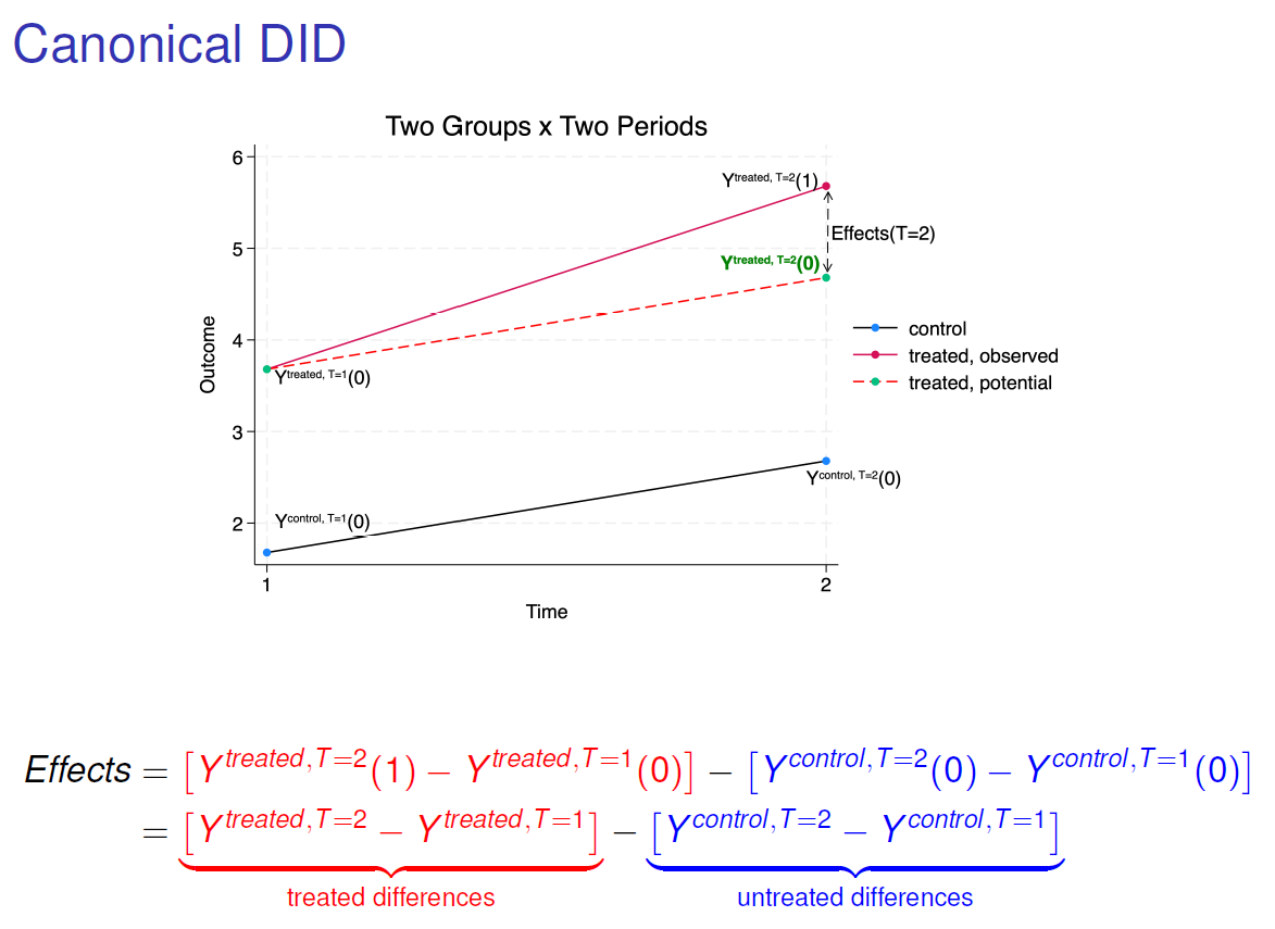
Basically, we will estimate the dotted red line, which not observed. It is the outcome in period 2 for the tread group if it did not received the treatment. We easily understand that this counterfactual situation is not observed, since the treated group… received the treatment in period 2.
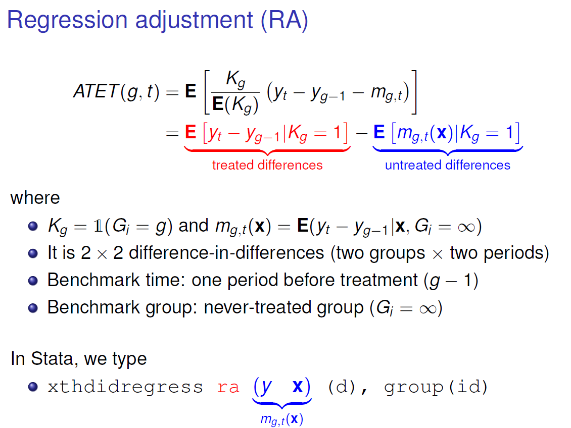
The first estimator (RA) will use information on the control group to estimate the information in the dotted red line, the untreated differences, with y the outcome, x and z are covariates, and d the treatment dummy. Besides, Gi = g indicates that the treatment started in time g for the group i. Gi = ∞ indicates that the group is the never-treated group.
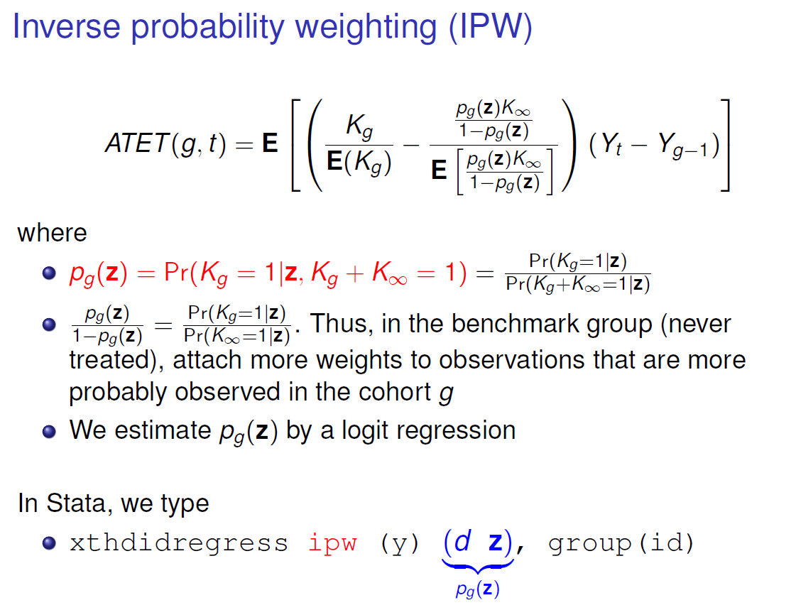
The second estimator (IPW) estimate the probability that the observation in the benchmark group belongs to the treated group to estimate the untreated differences:
The AIPW estimator combines the RA and IPW estimators:
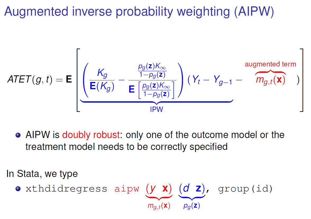
During the training, they recommend to start with IPW because it is doubly robust and use RA, if you have some extreme values in the weighting estimators.
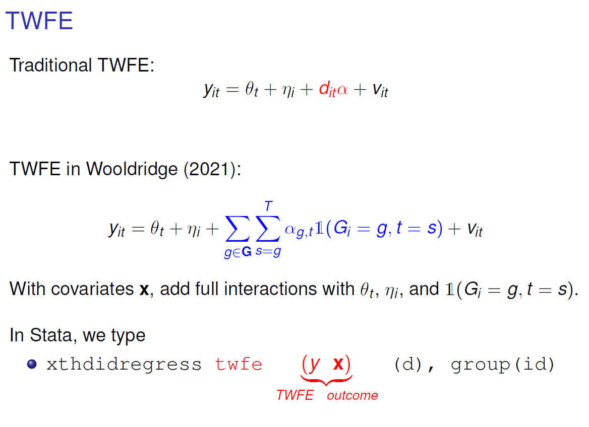
Finally, we have the TWFE estimator of Wooldridge (2021) that elegantly decomposes the dummy variable for the treatment dummy.
We have seen that estimating heterogeneous DID is now possible with Stata 18. These new commands offer very nice ways to visualize the ATET on several dimensions. The code for this example is available on my GitHub: https://github.com/.
References
Callaway, B., and P. H. C. Sant’Anna. 2021. Difference-in-differences with multiple time periods. Journal of Econometrics 225: 200–230. 12.001.
Wooldridge, J. M. 2021. Two-way fixed effects, the two-way Mundlak regression, and difference-in-differences estimators. Working
paper, Department of Economics, Michigan State University, East Lansing, MI. ssrn.3906345.