Estimating a nonlinear DSGE model with Stata

Today, I will show how to estimate a DSGE model with Stata in a few steps. The model consists of 8 equations and is a variant of the New Classical model presented in King and Rebelo (1999). It includes equations for output Y(t), consumption C(t), investment I(t), hours worked H(t), the interest rate R(t), the real wage W(t), the capital stock K(t), and productivity Z(t). Model variables must be weakly stationary. The model contains six parameters: α, β, χ, δ, ρ, and σ.

\begin{align}
\frac{1}{C_t} & =\beta E_t\left\{\left(\frac{1}{C_{t+1}}\right)\left(1+R_{t+1}-\delta\right)\right\} \\
\chi H_t & =\frac{W_t}{C_t} \\
Y_t & =C_t+I_t \\
Y_t & =Z_t K_t^\alpha H_t^{1-\alpha} \\
R_t & =\alpha \frac{Y_t}{K_t} \\
W_t & =(1-\alpha) \frac{Y_t}{H_t} \\
K_{t+1} & =I_t+(1-\delta) K_t \\
\ln \left(Z_{t+1}\right) & =\rho \ln \left(Z_t\right)+e_{t+1}
\end{align}

I reproduce here the description of the model in the (very complete) Stata Manual on DSGE: https://www.stata.com/manuals/dsge.pdf. Equation (1) is a consumption Euler equation that links consumption in the current period to expected future consumption and the expected future interest rate. Equation (2) is a labor supply equation that links hours worked to the wage and consumption. Equation (3) is a standard national income accounting identity, stating that output is split between consumption and investment. Equation (4) is an output supply equation or production function, stating that output is produced by combining capital K(t) and labor H(t) at productivity level Z(t). Equation (5) is a capital demand curve. Equation (6) is a labor demand curve. Equation (7) is the capital accumulation process. Equation (8) specifies a stochastic process for productivity. The stochastic shock e_t+1 is i.i.d. normal with mean zero and standard deviation σ_z.

The model includes six parameters. β is the discount factor reflecting a preference for current consumption relative to future consumption. α is a production parameter. χ is a preference parameter. δ is the depreciation rate. ρ measures the persistence of the stochastic productivity process. Finally, σ is the standard deviation of the innovations to the productivity process.

Now, we can bring the data for the US economy:

use https://www.stata-press.com/data/r18/usmacro2

save usmacro2.dta, replace

describe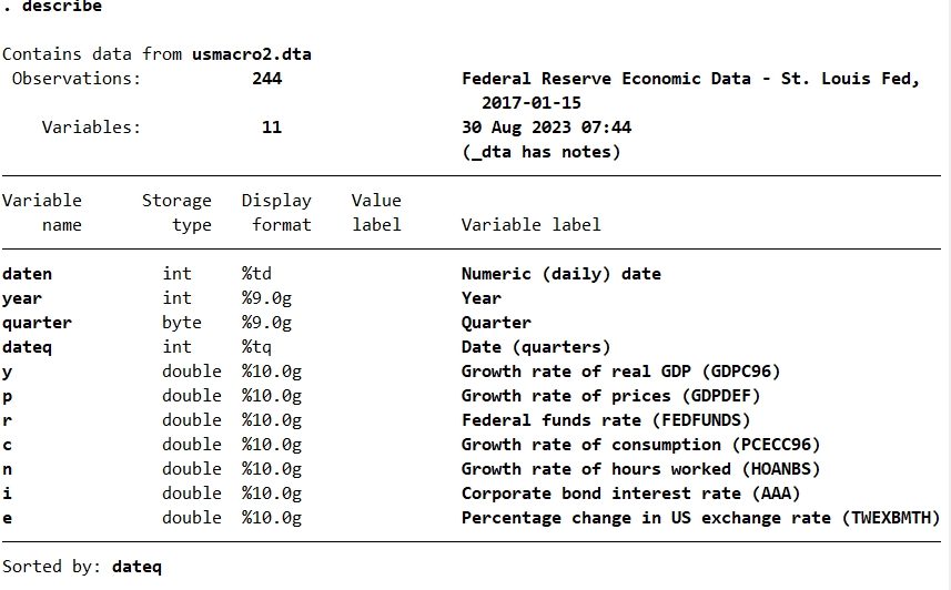

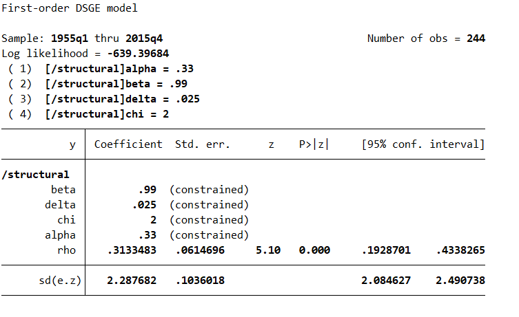
I now set the constrained parameters based on the paper of King and Rebelo (1999), basically we are using calibration. I will estimate the remaining parameters ρ and σ_z.

// Set the constraints

constraint 1 _b[alpha] = 0.33
constraint 2 _b[beta] = 0.99
constraint 3 _b[delta] = 0.025
constraint 4 _b[chi] = 2

dsgenl (1/c = {beta}*(1/F.c)*(1+F.r-{delta}))            ///
			({chi}*h = w/c)	                 ///
			(y = c + i)                      ///
			(y = z*k^{alpha}*h^(1-{alpha}))  ///
			(r = {alpha}*y/k)                ///
			(w = (1-{alpha})*y/h)            ///
			(F.k = i + (1-{delta})*k)        ///
			(ln(F.z) = {rho}*ln(z))          /// 
			, observed(y)                    ///
                        unobserved(c i r w h)            ///
                        exostate(z)                      ///
			endostate(k) constraint(1/4)

One way to understand the model is to find the state variables. Here, the state variables will have the F. operator and be at the left of the equal sign. In this example, it will be k and z. So, this model has 6 control variables (endogenous variables) and 2 state variables (exogenous variables). One of the state variables, F.z is modeled as a first-order autoregressive process. The state equation for F.k depends on the current value of a control variable, namely, i. Variables can be either observed (exist as variables in your dataset) or unobserved. Because the state variables are fixed in the current period, equations for state variables express how the one-step-ahead value of the state variable depends on current state variables and, possibly, current control variables.

Remember that the option exostate() lists all exogenous state variables, those that are subject to shocks. The option observed() lists observed control variables. The option unobserved() lists unobserved (latent) control variables. A fourth option, endostate(), is available for endogenous state variables, those that are not subject to shocks. State variables are always unobserved.

In the Stata help file, we have: “In the jargon, endogenous variables are called control variables, and exogenous variables are called state variables. The values of control variables in a period are determined by the system of equations. Control variables can be observed or unobserved. State variables are fixed at the beginning of a period and are unobserved. The system of equations determines the value of state variables one period in the future.”

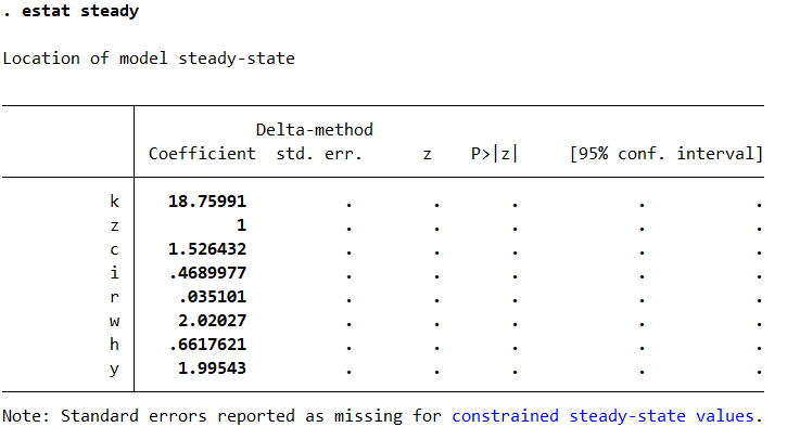
Then, I can solve the model to find the steady state:

estat steady

Afterwards, I can generate model implied covariance between variables:

estat covariance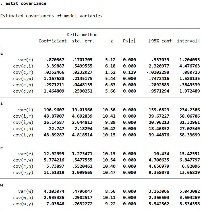

I draw impulse response functions for a productivity shock (obtained thanks to the state space form of the model, see the manual for more details) and I save the figure in the current directory. Note that the impulse–response graphs the response of model variables to a one-standard-deviation shock:

irf set rbcirf, replace

irf create est, step(20) replace

irf graph irf, impulse(z) response(y c i h w z)            ///
  byopts(yrescale)                                         ///
  ttitle(Effects of a Productivity shock (z))
  
graph rename prod, replace
graph export prod.png, replace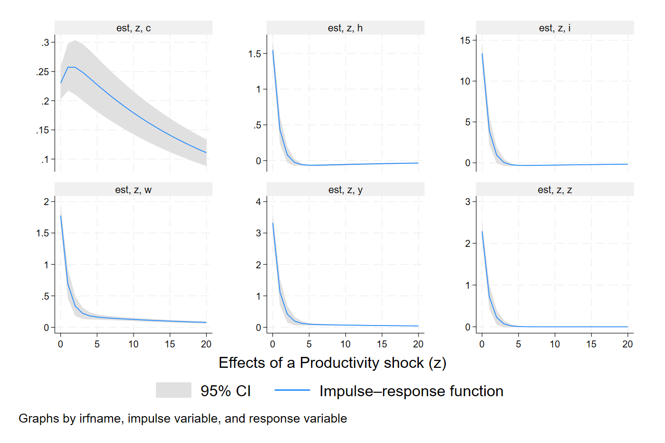

As mentioned in the Stata help file:

All model variables rise on a shock to productivity. For most model variables, the increase is short lived, and they return to their long-run values within five periods. Consumption is the exception (upper left panel). It rises smoothly for several periods, then gradually falls back to its long-run value.

As a final exercise, you can do a sensitivity exercise for a higher depreciation rate for the stock of capital. It would have been a counterfactual exercise if we have estimated the depreciation rate.

// Sentivity analyses (a higher rate for depreciation)

ereturn list

matrix list	e(b)

matrix b2 = e(b)

matrix b2[1,2] = 0.08

I change the second row of the matrix with the parameters:

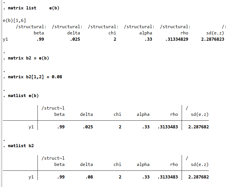
I estimate the model with the new value for the delta (see the new option in bold) and I create the IRFs, named counterfactual:

dsgenl (0 = {beta}*(c/F.c)*(1+F.r-{delta}) - 1)              ///
			(h = (1/{chi})*(w/c))		     ///
			(y = c + i)                                      ///
			(y = z*k^{alpha}*h^(1-{alpha}))                  ///
			(r = {alpha}*y/k)                                ///
			(w = (1-{alpha})*y/h)                            ///
			(F.k = i + (1-{delta})*k)                        ///
			(ln(F.z) = {rho}*ln(z))                          /// 
			, observed(y) unobserved(c i r w h) exostate(z)  ///
		        endostate(k) constraint(1 2 4) tech(nr) from(b2) ///
			solve
			
irf create counterfactual, step(20) replace
irf ograph (est z c irf) (counterfactual z c irf)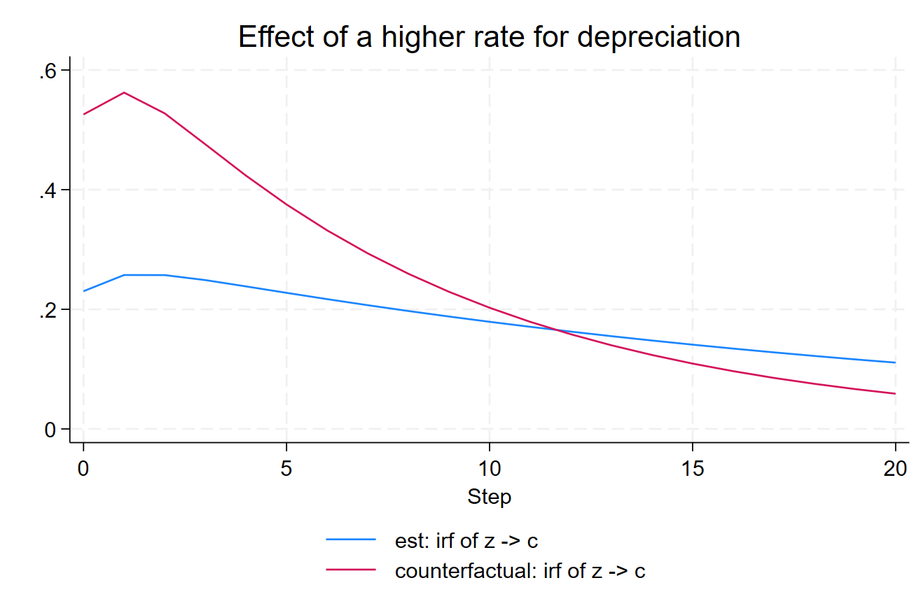

A higher depreciation rate makes that the effect on consumption of the productivity shock is higher. It helps you to understand the logic behind this particular model.

We have seen that the estimation of a Nonlinear New Classical model is possible in Stata. The dsgenl command is very flexible to estimate nonlinear DSGE models. The code for this example is available on my GitHub: https://github.com/JamelSaadaoui/EconMacroBlog

References

King, R. G., & Rebelo, S. T. (1999). Resuscitating real business cycles. Handbook of macroeconomics, 1, 927-1007.

David Schenck (2017). Estimating the parameters of DSGE models. Stata Blog, https://blog.stata.com/2017/07/11/estimating-the-parameters-of-dsge-models/

David Schenck (2017). Dynamic stochastic general equilibrium models for policy analysis, https://blog.stata.com/2018/04/23/dynamic-stochastic-general-equilibrium-models-for-policy-analysis/

StataCorp (2023). Stata dynamic stochastic general equilibrium models reference manual, https://www.stata.com/manuals/dsge.pdf