Natural Resources Economics with Mathematica

Today, let me draw your attention to a very interesting book: Natural Resource Economics. Analysis, Theory, and Applications by Jon M. Conrad, Cornell University, New York, Daniel Rondeau, University of Victoria, British Columbia.

The Economics of Natural Resources is a very important topic and uses several mathematical tools that are used in other areas of Economics. In the companion website for the book, you will find the Mathematica notebooks to answer the mathematical problems of each chapter. These are wonderful resources for students and researchers that want to use these mathematical tools. So please consider buying the book by yourself or by your institution.

We will focus on the chapter 1, which recalls the Fundamental concepts. The authors recall that “the study of optimal resources management shares methods and results with the field of macroeconomics, economic growth, and financial economics”.

Let us review the exercises for the Chapter 1, we have a two-period optimization problems, where t = 0 in the present period and t = 1 in the “future period,” can help develop economic intuition for more complex, multi-period problems, and they often permit analytic solutions for the optimal decisions that must be made in t = 0.

Exercise 1.1 of Chapter 1

The individual receives inheritance in the first period, t = 0, denoted by I₀ > 0. The individual will die in the second period, t = 1, and must determine consumption (c₀) and savings (s₀) in the first period so as to provide consumption in (c₁) the second period before dying. The utility function takes the form of a constant relative risk aversion, as you can see below,

U(c_t)=c_0^{(1-\eta)} /(1-\eta)

Saving in the first period is given by,

s_0=\left(I_0-c_0\right)\geq 0

The savings in the first period are invested, so they produce income in the second period with, r, the one-period rate of return on savings and r ∊ (0,1),

\left(I_0-c_0\right)(1+r)

In the second period, the individual consumes all his income, so I₁ = c₁. Let the one-period discount rate, δ, be positive, and, ρ, the one-period discount factor for utility be the following,

\rho=\frac{1}{1+\delta}

The optimization problem is the following:

\small 
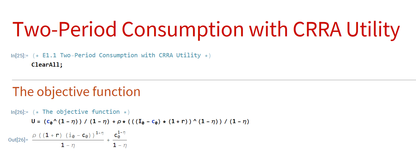
\underset{c_0}{\operatorname{Maximize{\space}}} U=c_0^{(1-\eta)} /(1-\eta)+\rho\left[\left(I_0-c_0\right)(1+r)\right]^{(1-\eta)} /(1-\eta)

In Mathematica, I enter the expression, after having cleared all the symbols;

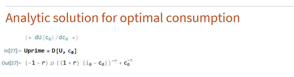
Then, I derive U with respect to c₀,

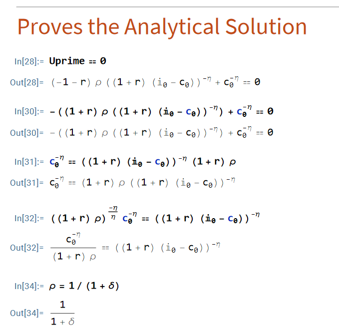
Then, I prove the analytic solution in the book starting from the derivative given by Mathematica,

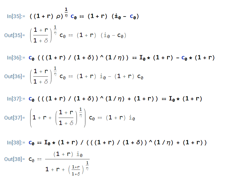
Finally, I obtain the optimal consumption for the first period using the analytic solution for defined values of the parameters and variables:

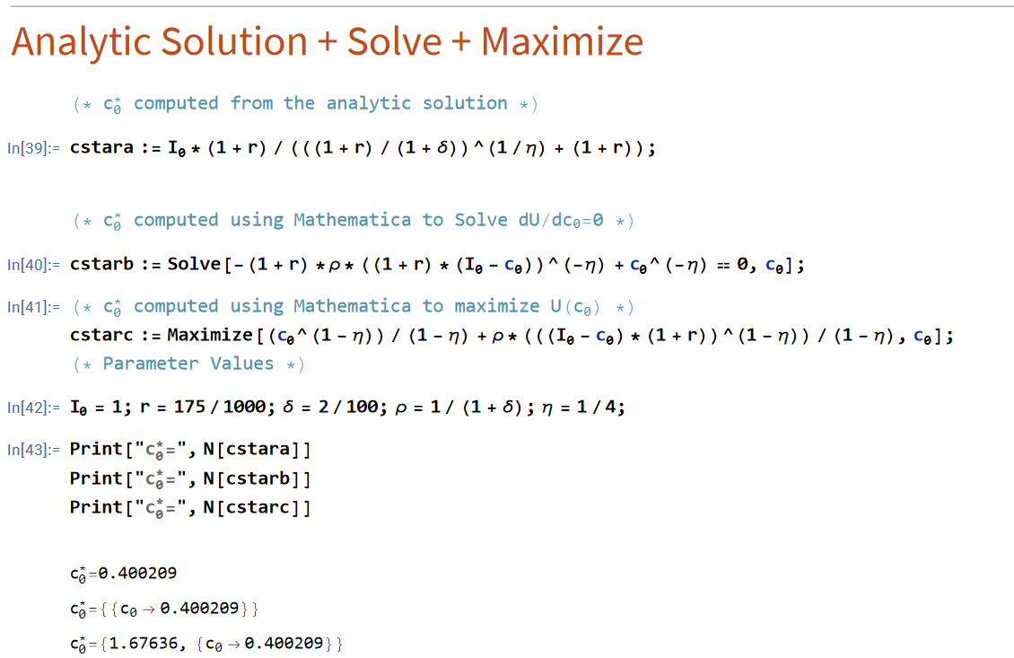
The optimal level of saving for the first period is equal to (I₀ – c₀ = 1 – 0.400209).

We have seen that Mathematica is a very powerful tool to solve two-period optimization problems. The code for this example is available on my GitHub: https://github.com/JamelSaadaoui/EconMacroBlog

References

Conrad, J. M., & Rondeau, D. (2020). Natural resource economics: analysis, theory, and applications. Cambridge University Press.
https://doi.org/10.1017/9781108588928