Estimate Non-Parametric Time-Varying Coefficients in Panel Data Models with Fixed Effects

Today, I will show you how to use the package of Ibrahima Amadou Diallo, xtnptimevar, that estimates non-parametric varying coefficients in panel data models with fixed effects. We are going to the data coming from the following paper, written with Linda Glawe and Can Xu, I recommend you to have a look:

Nonlinearities in the Inflation-Growth Relationship and the Role of Uncertainty: Evidence from China’s Provinces

Key takeaways

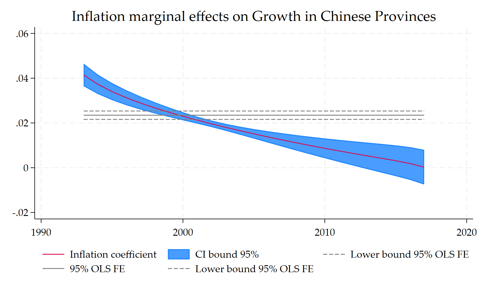
• Before 2012, lagged inflation had a positive marginal effect on growth.
• This is typical of developing countries where inflation is not a growth killer and is not associated with higher uncertainty.
• This pre-2012 configuration was similar to the case of France and Germany after WWII in the 1950s and in the 1960s.
• More generally, inflation becomes a growth killer after the countries reach a certain level of development and when the international context becomes more uncertain.
• This more uncertain context was due to the oil shock in the 1970s for France and Germany.
• For China, the post-GFC context and the growing geopolitical rivalry with the US generated a more uncertain context.

Let us start to dive into the Stata adaptation of Li, Chen and Gao’s (2011) corresponding original Matlab program.

This first part is a preparation to choose the folder and the scheme and other details. Finally, we install the package from SSC:

clear

use Glawe_Saadaoui_Xu_july2025.dta

set scheme stcolor

graph set window fontface "Palatino Linotype" 

global V C:\Users\jamel\Dropbox\stata\xtnptimevar

ssc install xtnptimevar

Then, we estimate the model and prepare some series to compare the time-varying and the constant coefficient on inflation:

**# Inflation-growth nexus in Chinese provinces

xtnptimevar g2_gdppc_const05_new L.slog_cpi_new, ///
stub(coefsi) bootstrap matsize(800) saving($V) forcereg

areg g2_gdppc_const05_new L.slog_cpi_new, a(unit_id)

gen n=_n

scalar sig = 0.1
	
generate b = .0234649 
generate se = .0011381
 
gen up = b + invnormal(1-sig/2)*se if _n <= 25
gen dn = b - invnormal(1-sig/2)*se if _n <= 25

Finally, we plot the graph with the help of addplot (see the following blogs on addplot).

tw ///
 rarea coefsi_cill_2 coefsi_ciul_2 coefsi_tvprime || ///
 line coefsi_b_2 coefsi_tvprime, ///
 ti(`"Inflation marginal effects on Growth in Chinese Provinces"') /// 
 xti("") name(INF, replace) ///
 legend(pos(6) col(3) ///
 order(2 "Inflation coefficient" ///
 1 "CI bound 95%"  ///
 3 "Lower bound 95% OLS FE" ///
 4 "95% OLS FE" ///
 5 "Lower bound 95% OLS FE"))
 
addplot: line up coefsi_tvprime if _n <= 25, ///
  lpattern(--) lcolor(gray) legend(pos(6) col(3) ///
 order(2 "Inflation coefficient" ///
 1 "CI bound 95%"  ///
 3 "Lower bound 95% OLS FE" ///
 4 "95% OLS FE" ///
 5 "Lower bound 95% OLS FE"))
addplot: line b coefsi_tvprime if _n <= 25, ///
  lpattern(solid) lcolor(gray) legend(pos(6) col(3) ///
 order(2 "Inflation coefficient" ///
 1 "CI bound 95%"  ///
 3 "Lower bound 95% OLS FE" ///
 4 "95% OLS FE" ///
 5 "Lower bound 95% OLS FE"))
addplot: line dn coefsi_tvprime if _n <= 25, ///
  lpattern(--) lcolor(gray)  legend(pos(6) col(3) ///
 order(2 "Inflation coefficient" ///
 1 "CI bound 95%"  ///
 3 "Lower bound 95% OLS FE" ///
 4 "95% OLS FE" ///
 5 "Lower bound 95% OLS FE"))

The results confirm that inflation was not a growth killer before 2012 in Chinese Provinces.

Conclusion

Inflation which is not associated with higher uncertain environment, is not a growth killer. I illustrated it with the help non-parametric varying coefficients model and in the context of Chinese provinces.

References

Ghosh, A., & Phillips, S. (1998). Warning: Inflation may be harmful to your growth. Staff Papers, 45(4), 672-710.

Glawe, L., Saadaoui, J., & Xu, C. (2024). Nonlinearities in the Inflation-Growth Relationship and the Role of Uncertainty: Evidence from China’s Provinces. Available at SSRN 5067849. 

Li, D., Chen, J., & Gao, J. (2011). Non‐parametric time‐varying coefficient panel data models with fixed effects. The Econometrics Journal, 14(3), 387-408.