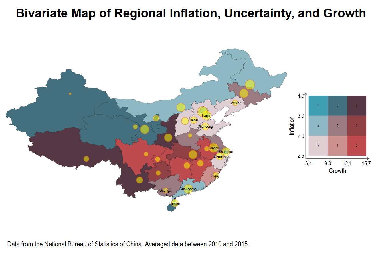
Let me show you how to add a third dimension on a bivariate maps in this second update of my blog on drawing bivariate maps for the Chinese regions. But, before I strongly recommend you to read my previous blogs on this topic. In particular, these two following blogs where I used Ben Jann’s geoplot Stata package:
Now, let us look at the result of this updated code with advanced options, we add circles to indicate the intensity of regional uncertainty:

Now let us look at the updated code where I underline the differences in bold. The only difference with the previous blog is that I need to create a new frame with the capital of the provinces. Besides, I add the circles for the provincial uncertainty in China using the data from: Yu, J., Shi, X., Guo, D. and Yang, L. (2021), ‘Economic policy uncertainty (EPU) and firm carbon emissions:
Evidence using a China provincial EPU index’, Energy Economics 94, 105071.
// New bimap version

/// New geoplot ///
use ne_10m_admin_1_states_provinces.dta,clear
merge 1:m _ID using "data/dataset_yearly_maps.dta", nogenerate
keep if year>= 2010
keep if year<= 2015
keep if iso_a2 == "CN"
generate g2_gdppc_const05_new100=g2_gdppc_const05_new*100
sort unit_id year
by unit_id: egen growth = mean(g2_gdppc_const05_new100)
by unit_id: egen inflation = mean(cpi_new)
by unit_id: egen uncertainy = mean(epu)
*keep if iso_a2 == "CN" | iso_a2 == "TW"
keep if year==2015
save ne_10m_admin_1_states_provinces_bis.dta, replace
/// New geoplot ///

geoframe create regions ///
 ne_10m_admin_1_states_provinces_bis.dta, id(_ID) ///
 coord(_CX _CY) ///
 shp(ne_10m_admin_1_states_provinces_shp.dta) ///
 replace
/// Replace shpfile() by shp()

geoframe describe regions

frame change regions

// Use the populated place file
// ne_10m_populated_places.dta
// and keep China with
// the iso_a2 code to create
// ne_10m_populated_places_CN.dta

// Merge uncertainy data in the ne_10m_populated_places_CN.dta
*merge_uncertainty_oct24.do

geoframe create towns ///
 ne_10m_populated_places_CN_uncertainy.dta, id(_ID) ///
 coord(_CX _CY) ///
 shp(ne_10m_populated_places_shp.dta) ///
 replace

*geoframe describe towns

*preserve
 bimap inflation growth, frame(regions) cut(pctile) ///
 palette(bluered)  ///
 title("{fontface Arial Bold:Bivariate Map of Regional Inflation, Uncertainty, and Growth}") ///
 note("Data from the National Bureau of Statistics of China. Averaged data between 2010 and 2015.") ///
 textx("Growth") texty("Inflation") texts(3.5) textlabs(3) values count ///
 ocolor(black) osize(0.05) ///
 polygon(data("ne_10m_admin_0_countries_shp") ///
 select(keep if _ID==189) ocolor(black) osize(0.05)) ///
 vallabs(1.8) ///
  geo((point towns [w = uncertainy] if FEATURECLA=="Admin-1 capital" | FEATURECLA=="Admin-0 capital", color(yellow%50) msize(0.75) mlcolor(red)) ///
 (label towns name if coastal==1, size(vsmall) color(black)))
*restore

graph rename Graph bimap2010_15_oct, replace

graph export bimap2010_15_oct.pdf, as(pdf) replace
graph export bimap2010_15_oct.png, as(png) replace
For illustrative purposes, I also add the code for the selection of regional capital and name adjustment between the region frame and the town frame:
clear

use ne_10m_populated_places_CN.dta, clear

keep if FEATURECLA=="Admin-1 capital" | ///
 FEATURECLA=="Admin-0 capital"

// Use FEATURECLA=="Admin-0 capital" to keep Beijing

rename ADM1NAME name

order name, first

replace name = "Ningxia" if name == "Ningxia Hui"
replace name = "Xinjiang" if name == "Xinjiang Uygur"
replace name = "Qinghai" if NAME == "Xining"
replace name = "Inner Mongol" if name == "Nei Mongol"

// drop duplicates capital of the regions
*drop in 5/5
drop if NAME == "Zhaotang"
drop if NAME == "Fushun"

merge 1:1 name using ne_10m_admin_1_states_provinces_bis.dta

save ne_10m_populated_places_CN_uncertainy.dta, replace
The files for the populated places are available on the Natural Earth website:
More details on how to draw maps for Chinese regions:
1 Comment
[…] Bivariate Maps for Chinese Regional Data (Second update) Drawing Maps for East Asia and Pacific Region […]