“Data! Data! Data!” he cried impatiently. “I can’t make bricks without clay.”
Sherlock Holmes.
The Adventure of the Copper Beeches, Sir Arthur Conan Doyle (1892).
In my previous post, I tried to explain in the simplest way Burgernomics. Here I reproduce the R code and the graphs used in the Big Mac Index made by the Economist.
For the July 2020 update, there are two source files (Comma-separated values format):
R Script for the results
# Generate data for the Big Mac Index

setwd("C:/Users/EconJamel/R/big-mac-data-2020-07")

library('tidyverse')
library('data.table')
library(dplyr)
library(magrittr)
library(ggplot2)

big_mac_countries = c('ARG', 'AUS', 'BRA', 'GBR', 'CAN', 'CHL', 'CHN', 'CZE', 'DNK',
                      'EGY', 'HKG', 'HUN', 'IDN', 'ISR', 'JPN', 'MYS', 'MEX', 'NZL',
                      'NOR', 'PER', 'PHL', 'POL', 'RUS', 'SAU', 'SGP', 'ZAF', 'KOR',
                      'SWE', 'CHE', 'TWN', 'THA', 'TUR', 'ARE', 'USA', 'COL', 'CRI',
                      'PAK', 'LKA', 'UKR', 'URY', 'IND', 'VNM', 'GTM', 'HND', #VNZ
                      'NIC', 'AZE', 'BHR', 'HRV', 'JOR', 'KWT', 'LBN', 'MDA', 'OMN',
                      'QAT', 'ROU', 'EUZ')
base_currencies = c('USD', 'EUR', 'GBP', 'JPY', 'CNY')

#NB: Venezuela removed.

# Data importation.

big_mac_data = fread('./source-data/big-mac-source-data.csv', na.strings = '#N/A',
                     # sort by date and then by country name, for easy reading;
                     # index on currency_code for faster joining
                     key = 'date,name', index = 'currency_code') %>%
  # remove lines where the local price is missing
  .[!is.na(local_price)]
tail(big_mac_data)

latest_date = big_mac_data$date %>% max
latest_date

# Raw index.

big_mac_data[, dollar_price := local_price / dollar_ex]
tail(big_mac_data)

big_mac_index = big_mac_data[
    !is.na(dollar_price) & iso_a3 %in% big_mac_countries
    ,.(date, iso_a3, currency_code, name, local_price, dollar_ex, dollar_price)]

for(currency in base_currencies) {
  big_mac_index[
    ,
    (currency) := dollar_price / .SD[currency_code == currency]$dollar_price - 1,
    by=date
  ]
}
big_mac_index[, (base_currencies) := lapply(.SD, round, 3L), .SDcols=base_currencies]
tail(big_mac_index)

to_plot = big_mac_index[date == latest_date]
to_plot$name = factor(to_plot$name, levels=to_plot$name[order(to_plot$USD)])
ggplot(to_plot[, over := USD > 0], aes(x=name, y=USD, color=over)) +
  geom_hline(yintercept = 0) +
  geom_linerange(aes(ymin=0, ymax=USD)) +
  geom_point() +
  coord_flip()

fwrite(big_mac_index, './output-data/big-mac-raw-index.csv')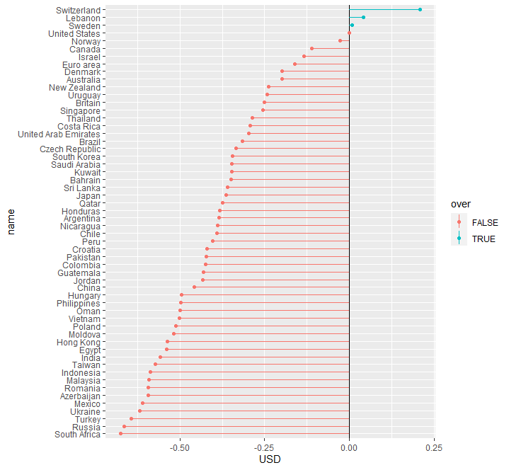
# GDP-adjusted index.

big_mac_gdp_data = big_mac_data[GDP_dollar > 0]

regression_countries = c('ARG', 'AUS', 'BRA', 'GBR', 'CAN', 'CHL', 'CHN', 'CZE', 'DNK',
                         'EGY', 'EUZ', 'HKG', 'HUN', 'IDN', 'ISR', 'JPN', 'MYS', 'MEX',
                         'NZL', 'NOR', 'PER', 'PHL', 'POL', 'RUS', 'SAU', 'SGP', 'ZAF',
                         'KOR', 'SWE', 'CHE', 'TWN', 'THA', 'TUR', 'USA', 'COL', 'PAK',
                         'IND', 'AUT', 'BEL', 'NLD', 'FIN', 'FRA', 'DEU', 'IRL', 'ITA',
                         'PRT', 'ESP', 'GRC', 'EST')
big_mac_gdp_data = big_mac_gdp_data[iso_a3 %in% regression_countries]

head(big_mac_gdp_data)

ggplot(big_mac_gdp_data, aes(x=GDP_dollar, y=dollar_price)) +
  facet_wrap(~date) +
  geom_smooth(method = lm, color='tomato') +
  geom_point(alpha=0.5)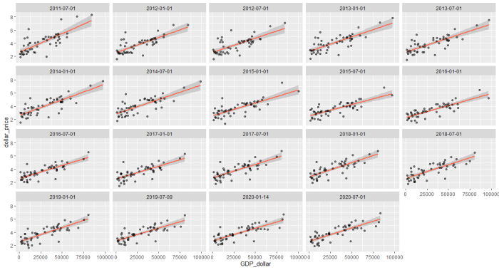
big_mac_gdp_data[,adj_price := lm(dollar_price ~ GDP_dollar)$fitted.values, by=date]
tail(big_mac_gdp_data)

ggplot(big_mac_gdp_data, aes(x=GDP_dollar, y=dollar_price)) +
  facet_wrap(~date) +
  geom_smooth(method = lm, color='tomato') +
  geom_linerange(aes(ymin=dollar_price, ymax=adj_price), color='royalblue', alpha=0.3) +
  geom_point(alpha=0.1) +
  geom_point(aes(y=adj_price), color='royalblue', alpha=0.5)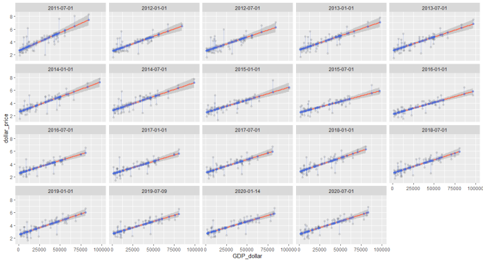
big_mac_adj_index = big_mac_gdp_data[
  !is.na(dollar_price) & iso_a3 %in% big_mac_countries
  ,.(date, iso_a3, currency_code, name, local_price, dollar_ex, dollar_price, GDP_dollar, adj_price)]

for(currency in base_currencies) {
  big_mac_adj_index[
    ,
    (currency) := (dollar_price / adj_price) /
      .SD[currency_code == currency, dollar_price / adj_price] - 1,
    by=date
  ]
}
big_mac_adj_index[, (base_currencies) := lapply(.SD, round, 3L), .SDcols=base_currencies]
tail(big_mac_index)

to_plot = big_mac_adj_index[date == latest_date]
to_plot$name = factor(to_plot$name, levels=to_plot$name[order(to_plot$USD)])
ggplot(to_plot[, over := USD > 0], aes(x=name, y=USD, color=over)) +
  geom_hline(yintercept = 0) +
  geom_linerange(aes(ymin=0, ymax=USD)) +
  geom_point() +
  coord_flip()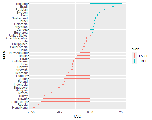
fwrite(big_mac_adj_index, './output-data/big-mac-adjusted-index.csv')

big_mac_full_index = merge(big_mac_index, big_mac_adj_index,
  by=c('date', 'iso_a3', 'currency_code', 'name', 'local_price', 'dollar_ex', 'dollar_price'),
  suffixes=c('_raw', '_adjusted'),
  all.x=TRUE
  )

fwrite(big_mac_full_index, './output-data/big-mac-full-index.csv')
R Script for exporting to Excel
# This script generates the Excel file for download
install.packages("devtools")
devtools::install_github("kassambara/r2excel")
library('r2excel')
library('magrittr')
library('data.table')

setwd("C:/Users/EconJamel/R/big-mac-data-2020-07")

data = fread('./output-data/big-mac-full-index.csv') %>%
    .[, .(
        Country = name,
        iso_a3,
        currency_code,
        local_price,
        dollar_ex,
        dollar_price,
        dollar_ppp = dollar_ex * dollar_price / .SD[currency_code == 'USD']$dollar_price,
        GDP_dollar,
        dollar_valuation = USD_raw * 100,
        euro_valuation = EUR_raw * 100,
        sterling_valuation = GBP_raw * 100,
        yen_valuation = JPY_raw * 100,
        yuan_valuation = CNY_raw * 100,
        dollar_adj_valuation = USD_adjusted * 100,
        euro_adj_valuation = EUR_adjusted * 100,
        sterling_adj_valuation = GBP_adjusted * 100,
        yen_adj_valuation = JPY_adjusted * 100,
        yuan_adj_valuation = CNY_adjusted * 100
    ), by=date]

dates = data$date %>% unique

wb = createWorkbook(type='xls')

for(sheetDate in sort(dates, decreasing = T)) {
    dateStr = sheetDate %>% strftime(format='%b%Y')
    sheet = createSheet(wb, sheetName = dateStr)
    xlsx.addTable(wb, sheet, data[date == sheetDate, -1], row.names=FALSE, startCol=1)
}

saveWorkbook(wb, paste0('./output-data/big-mac-',max(dates),'.xls'))
I get the following file that gather all the previous results:
3 Comments
Hi All,
I am running the Big Mac index code and consistently get the attached error! I am new to R and not sure what I am doing wrong as I have copied the code as is and only changed the location of where R should read the CSV from as it is saved on my laptop.
[]
Would really appreciate any assistance. I am very interested in the Big Mac index from an economics point of view
Thanks for your interest, I made a newer version of the R code here: big-mac-data-2020-07.zip
[…] Burgernomics: R codes and datasets July 20, 2020 […]