From Eurostat to a Monthly Inflation Panel in Stata

Eurostat spreadsheets are designed to be read by people, but their layout is not always immediately suitable for panel-data analysis. In the monthly inflation workbook used here, countries are stored in rows, months are stored across hundreds of columns, and almost every monthly value is followed by a separate observation-flag column. The difficult part is therefore not the statistical calculation. It is translating this alternating Excel structure into variable names that Stata can reshape.

This tutorial works with one specific Eurostat extract: the monthly Harmonised Index of Consumer Prices (HICP) dataset prc_hicp_minr, downloaded as prc_hicp_minr__custom_22342827_spreadsheet.xlsx. The selected series is the total HICP index under ECOICOP version 2, expressed with 2015 = 100, from January 1996 to July 2026. The objective is to construct a monthly country panel containing the HICP index and a calculated year-on-year inflation rate.

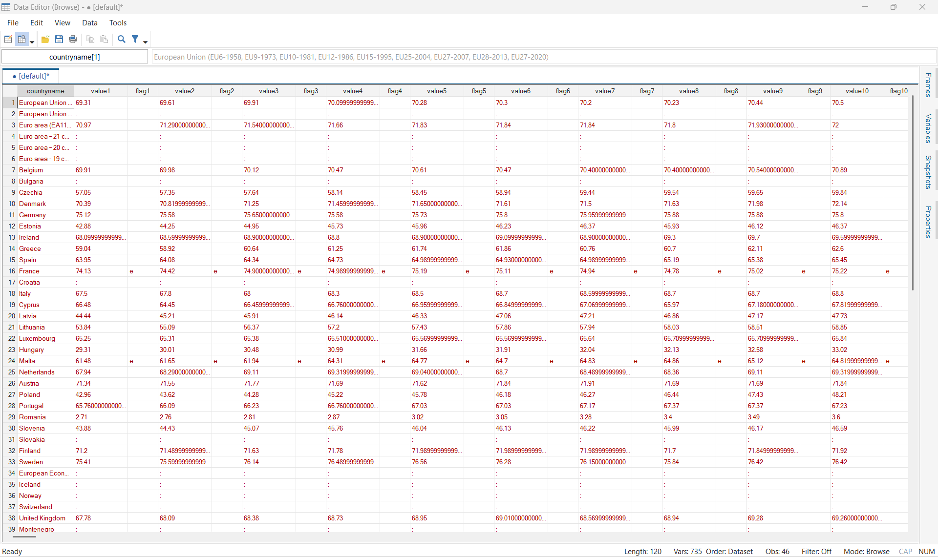
The central part of the post is the 367-iteration loop. I explain every instruction in that loop, including how Stata stores the original variable names, how it retrieves a variable by its position, and why the final flag variable has to be created separately.

1. The exact Eurostat extract

The source is Eurostat’s monthly HICP indices and rates-of-change dataset, identified by the code prc_hicp_minr. For this exercise, the Data Browser selection was restricted to one monthly series:

Dimension	Selection used in this extract
Frequency	Monthly
Classification	ECOICOP version 2
Product aggregate	Total HICP
Unit	Index, 2015 = 100 (I15)
Time coverage	January 1996–July 2026
Downloaded file	prc_hicp_minr__custom_22342827_spreadsheet.xlsx

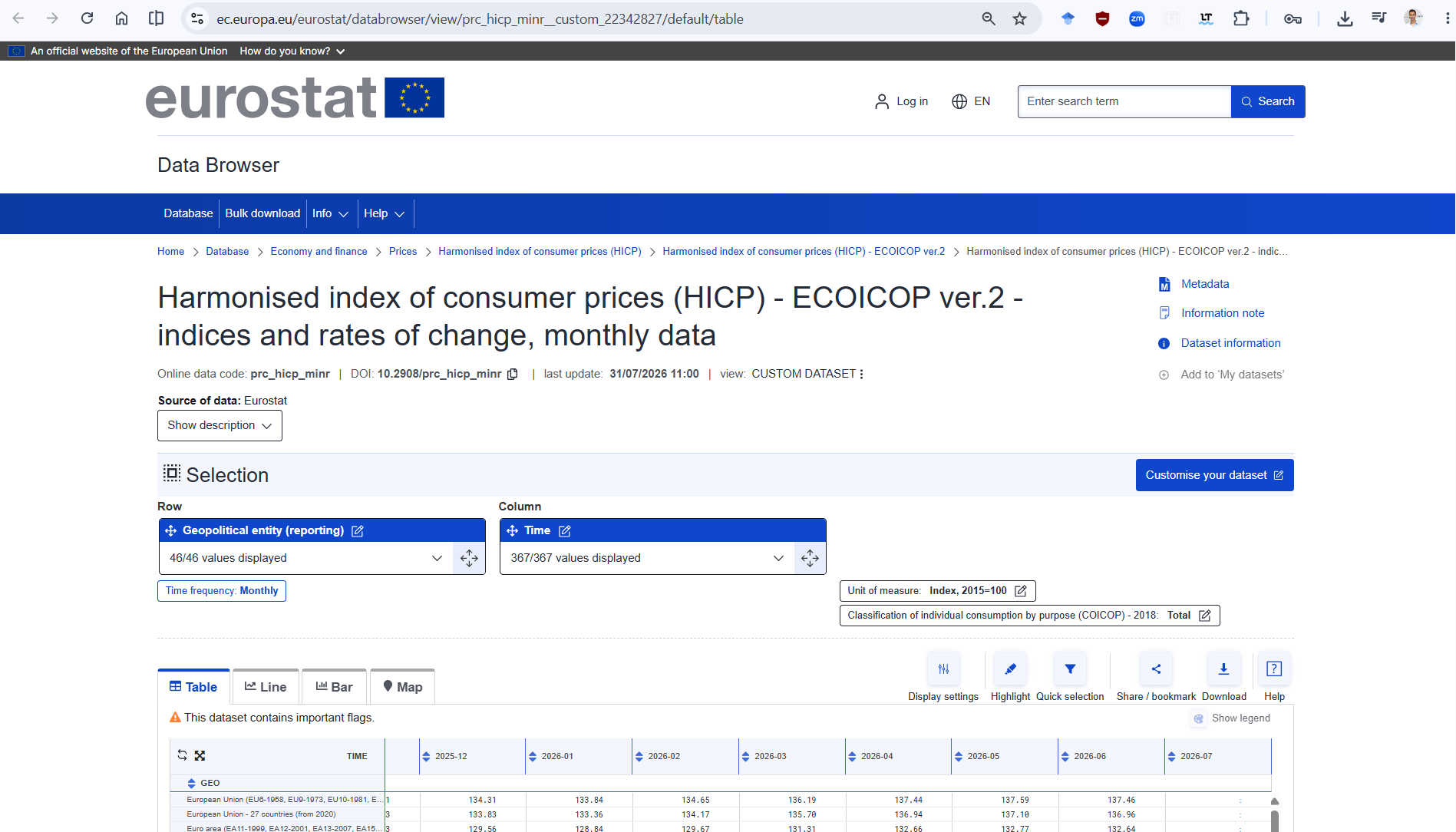
Eurostat changed the common HICP reference period to 2025 = 100 in 2026, but its database continues to provide both 2025 = 100 and 2015 = 100 indices. This particular workbook uses the 2015 = 100 series, so the variable label in the Stata code must retain that reference. Eurostat documents the available monthly indices and the 2026 methodological changes on its HICP information page. The dimensions of the worked selection can also be checked through Eurostat’s official filtered API response.

The Excel layout used below also depends on a specific download option: flags were kept on the same worksheet as their associated values. Eurostat’s Data Browser download guide explains that selecting “Add flags as a separate sheet” produces a different workbook. The loop in this post applies to the same-sheet layout.

2. Inspecting the workbook structure

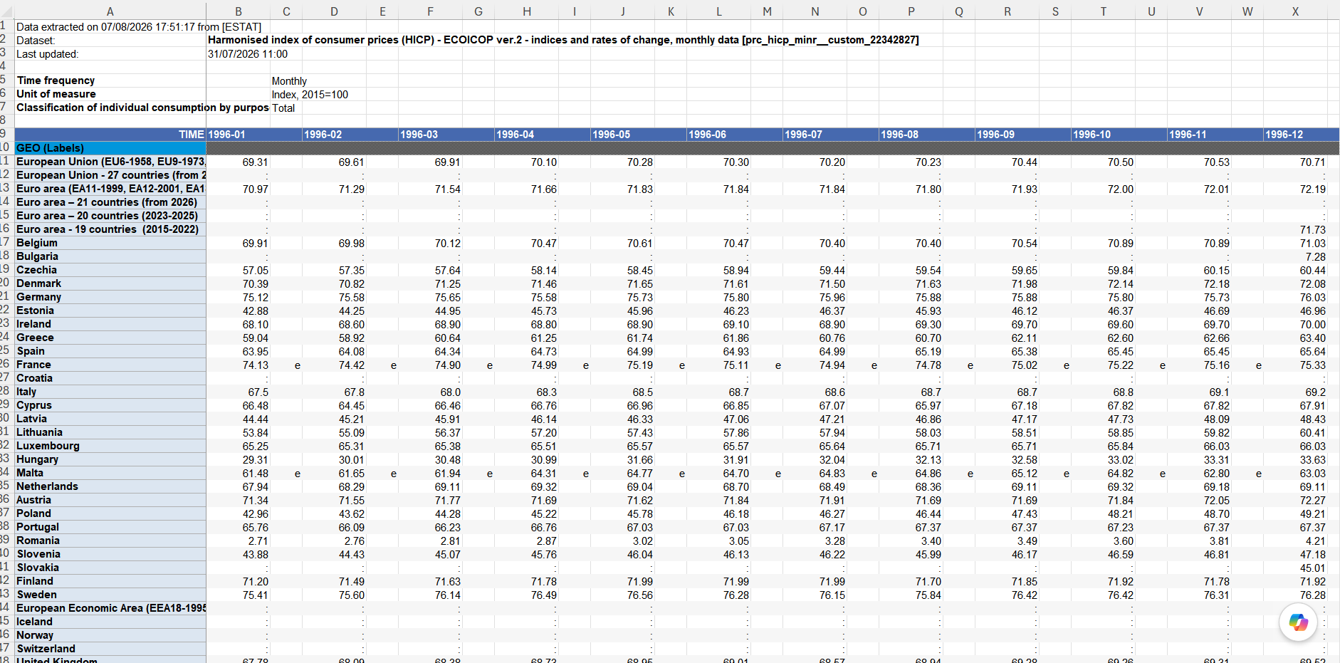
The data occupy Sheet 1, in the range A11:ABF56. This range has 46 rows and 734 columns:

• column A contains the geography name;
• columns B, D, F, and so on contain monthly HICP values;
• columns C, E, G, and so on contain the corresponding Eurostat flags;
• the final column, ABF, contains the July 2026 value;
• the entirely empty July 2026 flag column is absent.

The beginning of the worksheet therefore follows this pattern:

Position in Stata	Excel column	Content
1	A	Country or geography name
2	B	January 1996 HICP value
3	C	January 1996 flag
4	D	February 1996 HICP value
5	E	February 1996 flag
6	F	March 1996 HICP value
7	G	March 1996 flag

There are exactly 367 monthly positions from January 1996 to July 2026:

(2026 − 1996) × 12 + (7 − 1) + 1 = 367.

If every month had both a value column and a flag column, the workbook would contain:

1 country column + 367 value columns + 367 flag columns = 735 columns.

In the actual range there are only 734 columns because the last flag column is entirely empty and is not present:

1 + 367 + 366 = 734.

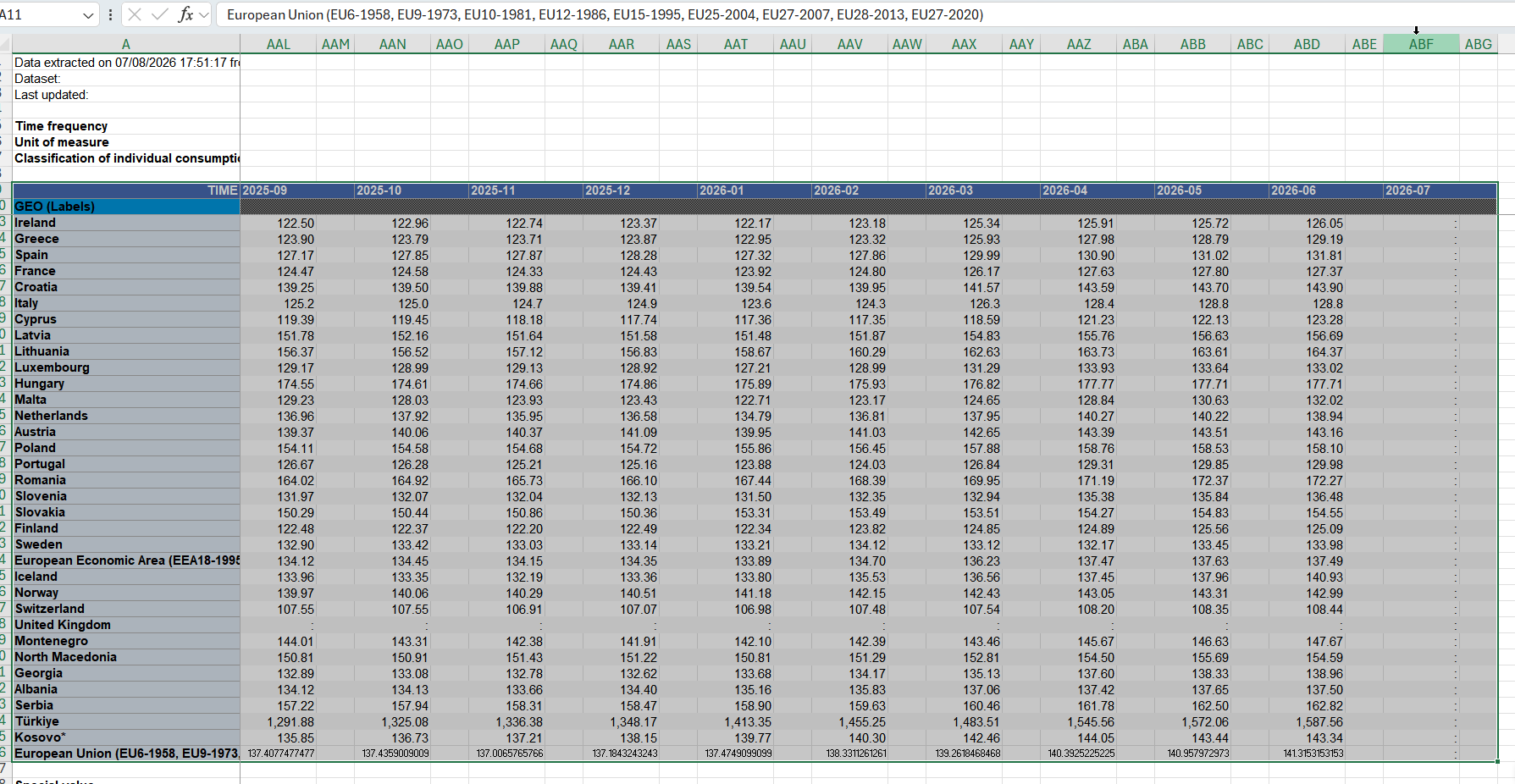
This single missing column explains the special treatment of flag367 later in the code.

3. Importing the Excel range as strings

import excel ///
"DATA\prc_hicp_minr__custom_22342827_spreadsheet.xlsx", ///
sheet("Sheet 1") ///
cellrange(A11:ABF56) ///
allstring clear

rename A countryname

Each option has a precise role:

• sheet("Sheet 1") selects the worksheet containing the data.
• cellrange(A11:ABF56) imports only the 46-by-734 rectangle used in this extract.
• allstring imports every Excel column as a string variable. This is important because the worksheet mixes numerical index values, the colon used for unavailable observations, and textual status flags.
• clear replaces the dataset currently in Stata’s memory.

The command does not use firstrow. Stata therefore assigns the Excel column letters as variable names: A, B, C, and so on. The first instruction after the import gives the identifier a meaningful name:

rename A countryname

Before running the loop, it is useful to confirm that the imported file really has the expected structure:

describe, short
ds
list countryname B C D E F G in 1/5, noobs clean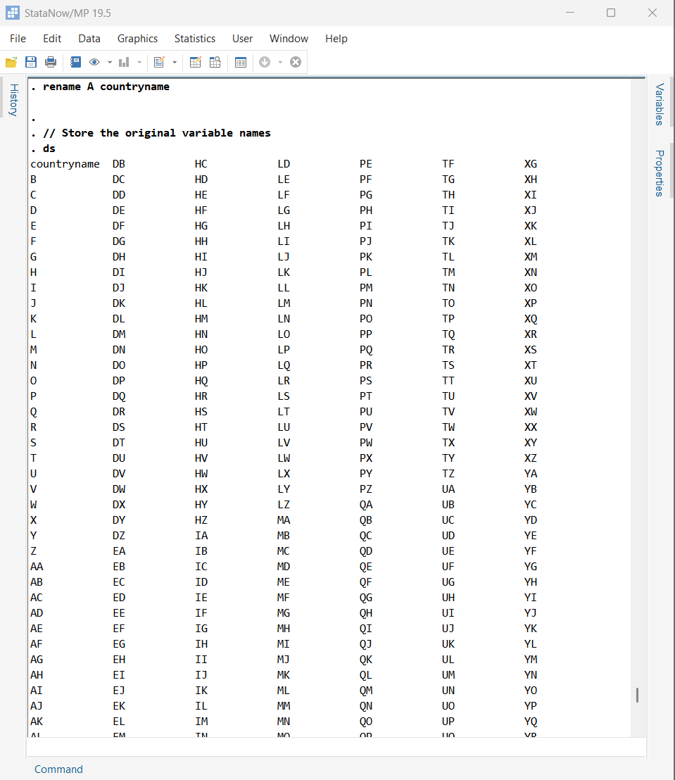

The list should show a country name followed by a monthly value, its flag, the next monthly value, its flag, and so forth. The loop relies entirely on this ordering. It does not read the calendar labels from Excel.

4. Why the variables must be renamed before reshape

Stata’s reshape long command recognizes repeated variables through a common stub and a numerical suffix. The imported Excel names do not have that structure:

countryname  B  C  D  E  F  G  ...  ABF

We need to turn them into:

countryname  value1  flag1  value2  flag2  value3  flag3  ...  value367  flag367

The words value and flag will be the two stubs. The suffixes from 1 to 367 will identify the monthly position. Once those names exist, reshape can move the suffix into a new variable called mindex.

5. The value–flag loop, line by line

This is the central block:

// Store the original variable names
ds
local variables `r(varlist)'

// 367 months from January 1996 to July 2026
forvalues j = 1/367 {

    local value_column = 2 * `j'
    local old_value : word `value_column' of `variables'

    rename `old_value' value`j'

    // The final flag column is absent because it is entirely empty
    if `j' < 367 {

        local flag_column = 2 * `j' + 1
        local old_flag : word `flag_column' of `variables'

        rename `old_flag' flag`j'
    }
}

// Add the absent flag variable for July 2026
generate str1 flag367 = ""

5.1 ds records the variables in their current order

ds

The command ds lists the variables in the dataset. More importantly for this program, it leaves the ordered list of variable names in the returned result r(varlist).

Immediately after the import and the renaming of A, that returned list begins as follows:

countryname B C D E F G ... ABF

There are 734 words in this list because each variable name counts as one word.

5.2 The local macro freezes the original names

local variables `r(varlist)'

This instruction copies the contents of r(varlist) into a local macro named variables. In simplified form, Stata behaves as if it had executed:

local variables countryname B C D E F G ... ABF

A local macro is temporary text stored in memory while the do-file or program is running. To ask Stata to substitute its contents, the macro name is enclosed between a left backtick and a right apostrophe:

`variables'

Saving this list before the loop is essential because the loop will progressively rename B, C, D, and all the remaining imported variables. The local macro remains a snapshot of the original names. For example, after B has become value1, word 2 in variables is still the text B.

It is also good practice to copy r(varlist) immediately. Returned results beginning with r() can be replaced by a later r-class command.

For this fixed extract, the number of stored names can be used as a diagnostic without changing the loop:

local nvars : word count `variables'
display as text "Number of imported variables: `nvars'"

if `nvars' != 734 {
    display as error "Expected 734 imported variables; found `nvars'."
    exit 459
}

: word count counts the words in the stored list, so it counts the imported variables. The test stops the do-file if a later workbook has a different width. It is only a consistency check: the fixed number 367 still controls the dataset-specific loop.

5.3 forvalues creates the monthly-position counter

forvalues j = 1/367 {

The loop creates a local macro called j. Its value is 1 in the first iteration, 2 in the second iteration, and so on until 367. Both endpoints are included.

The number 367 is fixed deliberately because this code is written for the exact January 1996–July 2026 workbook. Stata does not discover the dates here. The number was established by inspecting the Excel headers and confirming the column count. If a later download includes August 2026, both the imported range and the final loop bound must be updated.

The opening brace tells Stata where the repeated block begins. The matching closing brace tells it where that block ends.

5.4 Monthly values occupy the even positions

local value_column = 2 * `j'

The first variable, countryname, occupies position 1. The monthly values therefore occupy positions 2, 4, 6, and so on. Multiplying j by 2 produces exactly this sequence:

j	Calculation	value_column
1	2 × 1	2
2	2 × 2	4
3	2 × 3	6
367	2 × 367	734

The syntax local name = expression asks Stata to evaluate a numerical expression. Thus, when j is 2, the instruction expands to:

local value_column = 2 * 2

and the local macro value_column contains the number 4.

5.5 : word retrieves a variable name by position

local old_value : word `value_column' of `variables'

This line uses an extended macro function. Its general logic is:

local new_macro : word position of list

It selects one word from a list of words. Here, the list is the snapshot of the original variable names, and the requested position is stored in value_column.

Suppose that the loop is in its second iteration, so j=2. We already know that value_column=4. Stata therefore interprets the instruction as:

local old_value : word 4 of countryname B C D E F G ... ABF

The fourth word is D. The local macro old_value consequently contains the text D.

This point is fundamental: : word retrieves the name of a variable. It does not retrieve an HICP observation stored inside that variable.

5.6 The selected variable receives the value# name

rename `old_value' value`j'

There are two macro substitutions in this command. In the second iteration, old_value contains D and j contains 2. The line expands to:

rename D value2

The expression value`j' joins the literal text value to the current loop number. It creates value1, value2, …, value367.

5.7 Flags occupy the following odd positions

if `j' < 367 {

    local flag_column = 2 * `j' + 1
    local old_flag : word `flag_column' of `variables'

    rename `old_flag' flag`j'
}

For the first 366 months, every value is immediately followed by a flag. The flag positions are therefore 3, 5, 7, …, 733, which are generated by 2j+1.

In the second iteration:

1. j=2;
2. flag_column = 2 × 2 + 1 = 5;
3. word 5 in the original list is E;
4. old_flag therefore contains E;
5. the rename command expands to rename E flag2.

The condition if `j' < 367 is evaluated once in each loop iteration. It is a programming condition, not an if qualifier applied separately to the observations. For j=1 through j=366, the condition is true and Stata renames a flag. For j=367, it is false and Stata skips the entire flag block.

This condition prevents the code from requesting word 735 from a list that contains only 734 words.

5.8 The 367th iteration is intentionally different

The final iteration can be followed numerically:

• j = 367;
• value_column = 2 × 367 = 734;
• word 734 in the original variable list is ABF;
• rename `old_value' value`j' becomes rename ABF value367;
• 367 < 367 is false, so Stata does not look for a flag at position 735.

After the loop has finished, the July 2026 value exists as value367, but there is no flag367. The following instruction creates the empty partner variable:

generate str1 flag367 = ""

str1 defines a string variable that can hold one character. The expression "" is a missing string value in Stata. Every country therefore receives an empty July 2026 flag. This does not invent a Eurostat status; it explicitly records that no flag was supplied and completes the regular value#/flag# naming structure.

5.9 A complete trace of the loop

Iteration	Value action	Flag action
j=1	Position 2: B → value1	Position 3: C → flag1
j=2	Position 4: D → value2	Position 5: E → flag2
j=366	Position 732: ABD → value366	Position 733: ABE → flag366
j=367	Position 734: ABF → value367	Skipped; create empty flag367 after the loop

After the loop, the variables follow exactly the pattern needed for the next operation:

countryname value1 flag1 value2 flag2 ... value367 flag367

5.10 What the loop assumes

The loop is correct for this workbook because four facts were established before it was run:

1. countryname is the first and only identifier variable.
2. The first monthly value is in position 2.
3. Values and flags alternate without interruption through position 733.
4. The only absent flag is the final, entirely empty July 2026 flag.

The loop cannot discover a missing flag in the middle of the workbook. Such a missing column would shift every later assignment. This is why visually inspecting the beginning and end of the Excel extract is part of the data construction, not a cosmetic preliminary.

6. Reshaping the data from wide to long

reshape long value flag, i(countryname) j(mindex)

Stata now recognizes two stubs: value and flag. It takes the numerical suffixes from 1 to 367 and stores them in the new variable mindex. The wide structure becomes:

countryname	mindex	value	flag
Country A	1	January 1996 index	January 1996 flag
Country A	2	February 1996 index	February 1996 flag
Country A	3	March 1996 index	March 1996 flag

Because the imported range contains 46 geography rows and 367 monthly positions, the long dataset contains 46 × 367 = 16,882 geography-month rows before unavailable observations are dropped.

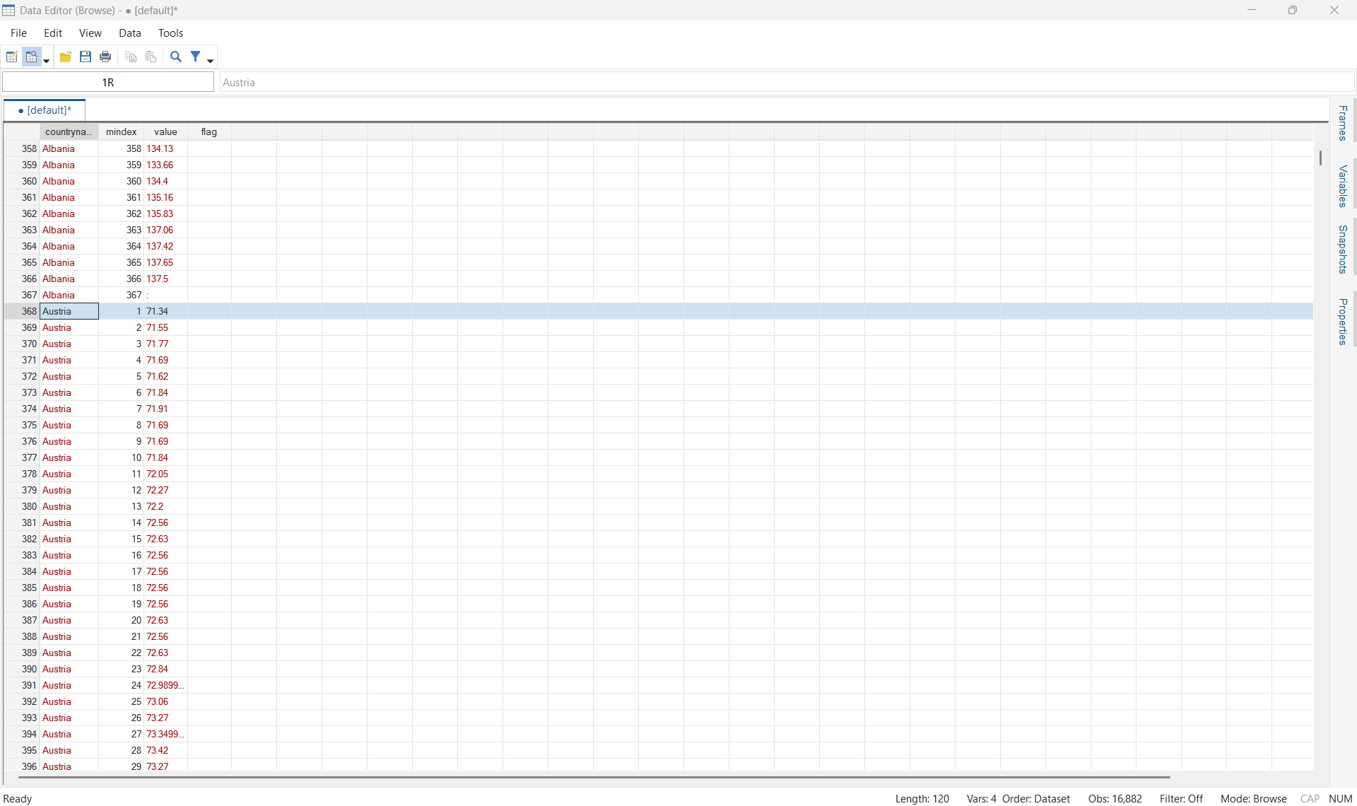
A useful immediate check is:

isid countryname mindex
list countryname mindex value flag in 1/12, noobs clean

The first command verifies that each country–position pair is unique. The second allows a direct comparison with the first monthly columns in the original workbook.

7. Constructing the monthly date

generate month = ym(1996,1) + mindex - 1
format month %tm

The variable mindex is only a sequence from 1 to 367. The function ym(1996,1) creates Stata’s internal monthly date for January 1996. Adding mindex-1 converts the sequence into consecutive calendar months:

• when mindex=1, the offset is 0 and the date is January 1996;
• when mindex=2, the offset is 1 and the date is February 1996;
• when mindex=367, the date is July 2026.

The subtraction of 1 is essential. Without it, the first observation would incorrectly be assigned to February 1996.

The format command changes only how the underlying monthly integer is displayed. It does not change its numerical value. The endpoints can be checked directly:

assert month == ym(1996,1) if mindex == 1
assert month == ym(2026,7) if mindex == 367
summarize month, format

8. Converting the index to numeric form

replace value = "" if value == ":"
destring value, replace

rename value hicp_index

label variable hicp_index ///
"Total HICP index, ECOICOP v2 (2015=100)"

drop if missing(hicp_index)

The variable value is still a string because the workbook was imported with allstring. In this extract, a colon denotes an unavailable observation. The first instruction replaces that colon with the empty string that Stata recognizes as a missing string value. The destring command can then convert the remaining index observations to numeric values. Eurostat’s format guide confirms that the colon means that no value is available.

The colon must never be recoded as zero. A zero would be treated as an observed price index and would produce meaningless inflation rates.

Before dropping unavailable observations, the data can be inspected with:

count if value == ":"
tabulate flag, missing
list countryname month value flag if value == ":" in 1/20, noobs clean

The observation flags should also be retained until their contents have been examined. They may convey information about the status of individual data points.

For this exact I15/TOTAL selection, the complete grid contains 16,882 country-or-aggregate–month positions. Of these, 14,583 contain an index value and 2,299 are unavailable. July 2026 exists as the 367th grid position, which is why the loop and date construction extend to July, but the July 2026 index values are unavailable in this extract. After drop if missing(hicp_index), the latest usable month is therefore June 2026. This is an important distinction between the coverage of the downloaded grid and the coverage of the usable observations.

9. Converting geography names into IMF country codes

kountry countryname, from(other) stuck marker

drop if MARKER == 0
drop MARKER

rename _ISO3N_ ISO3N

kountry ISO3N, from(iso3n) to(imfn)

rename _IMFN_ imfcode

kountry is a community-contributed Stata command that converts country identifiers between naming and coding systems. The first call converts the geography name to a numeric ISO code. The second converts that ISO code to an IMF numerical country code.

The option marker creates MARKER, which identifies whether the first conversion succeeded. It is important to inspect failed matches before deleting them:

list countryname if MARKER == 0, noobs clean

A failed match may be a regional aggregate that should be removed, but it may also be a country whose spelling differs from the crosswalk. In this extract, Czechia should be standardized before running kountry:

replace countryname = "Czech Republic" if countryname == "Czechia"

This line belongs before the first kountry command. Inspecting MARKER==0 prevents an otherwise valid country panel from being removed silently by drop if MARKER == 0.

The wildcard renaming instructions accommodate the variable names generated by kountry. After the two conversions, the variables that are no longer required are removed:

drop countryname mindex ISO3N

10. Declaring the monthly panel and calculating inflation

isid imfcode month
xtset imfcode month

generate inflation_yoy = ///
100 * (hicp_index / L12.hicp_index - 1)

isid imfcode month verifies that the combination of country and month uniquely identifies every remaining observation. If it fails, the problem must be investigated before proceeding.

xtset imfcode month tells Stata that imfcode identifies the panel and month identifies monthly time. This declaration is what gives the lag operator L12. its meaning.

The inflation formula is:

100 × (HICP(t) / HICP(t−12) − 1).

For each country, L12.hicp_index retrieves the index exactly 12 calendar months earlier. The first 12 available months of a continuous country series necessarily have missing year-on-year inflation because there is no corresponding observation one year earlier. An internal gap also produces a missing lag rather than using the previous row incorrectly.

Because both the current and lagged indices have the same reference base, rebasing the whole index does not change this percentage rate. However, Eurostat notes that rates calculated from published rounded indices can differ slightly from rates calculated from its higher-precision underlying figures. The series created here is therefore the year-on-year rate implied by the downloaded index.

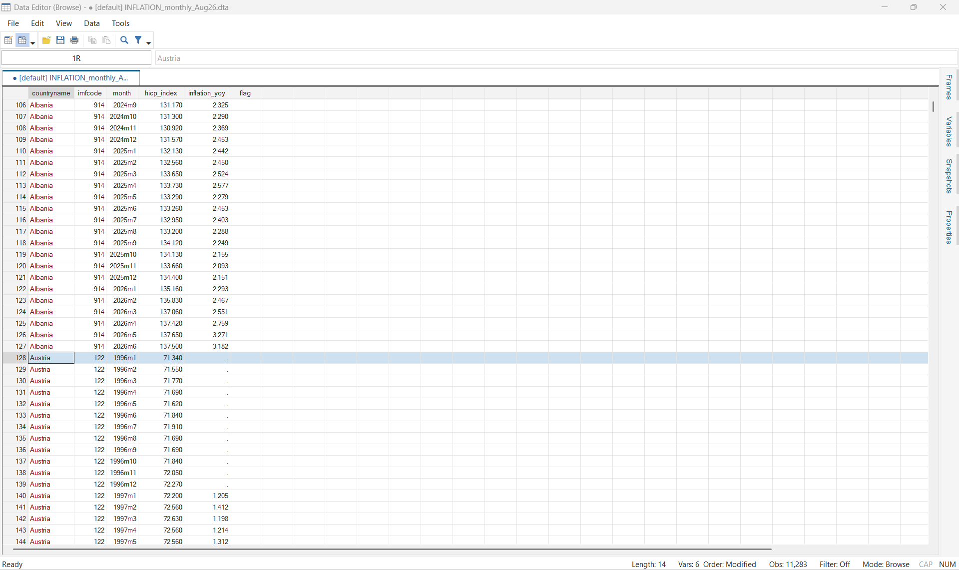
11. Inspecting and saving the final panel

The final commands format and organize the variables:

label variable inflation_yoy ///
"HICP inflation, year-on-year (%)"

format hicp_index inflation_yoy %9.3f

order imfcode month hicp_index inflation_yoy flag
sort imfcode month

summarize month, format
compress

save "DATA\INFLATION_monthly_Aug26.dta", replace

Before saving, a compact inspection can be added:

describe
xtdescribe
summarize hicp_index inflation_yoy, detail
misstable summarize hicp_index inflation_yoy
tabulate flag, missing
list imfcode month hicp_index inflation_yoy flag in 1/20, noobs clean

compress reduces the storage type where this can be done without losing information. It does not alter the substantive values. The resulting file contains one observation per IMF country code and month.

The main lesson is that the loop is a translation between two structures. Excel supplies a country column followed by alternating values and flags. Stata needs repeated stubs followed by common numerical suffixes. Once the positional logic has been made explicit, the wide-to-long transformation becomes straightforward and auditable.

12. Complete Stata code

// -----------------------------------------------------------------------------
**# Monthly HICP inflation
// Eurostat dataset: prc_hicp_minr
//
// ECOICOP version 2
// Total HICP index, 2015 = 100
// Coverage: January 1996–July 2026
// Original monthly frequency retained
// -----------------------------------------------------------------------------

import excel ///
"DATA\prc_hicp_minr__custom_22342827_spreadsheet.xlsx", ///
sheet("Sheet 1") ///
cellrange(A11:ABF56) ///
allstring clear

rename A countryname

// Store the original variable names
ds
local variables `r(varlist)'

// Verify the width of this exact extract
local nvars : word count `variables'
display as text "Number of imported variables: `nvars'"

if `nvars' != 734 {
    display as error ///
        "Expected 734 imported variables; found `nvars'."
    exit 459
}

// 367 months from January 1996 to July 2026
forvalues j = 1/367 {

    local value_column = 2 * `j'
    local old_value : word `value_column' of `variables'

    rename `old_value' value`j'

    // The final flag column is absent because it is entirely empty
    if `j' < 367 {

        local flag_column = 2 * `j' + 1
        local old_flag : word `flag_column' of `variables'

        rename `old_flag' flag`j'
    }
}

// Add the absent flag variable for July 2026
generate str1 flag367 = ""

// Transform from wide to long format
isid countryname
reshape long value flag, i(countryname) j(mindex)
isid countryname mindex

// Construct the monthly date
generate month = ym(1996,1) + mindex - 1
format month %tm

// Verify the reconstructed dates
assert month == ym(1996,1) if mindex == 1
assert month == ym(2026,7) if mindex == 367

// Inspect unavailable observations and flags
count if value == ":"
tabulate flag, missing

// Convert the HICP index into a numeric variable
replace value = "" if value == ":"
destring value, replace

rename value hicp_index

label variable hicp_index ///
"Total HICP index, ECOICOP v2 (2015=100)"

// Remove unavailable observations
drop if missing(hicp_index)

// Standardize the country name needed by the crosswalk
replace countryname = "Czech Republic" ///
    if countryname == "Czechia"

// Convert country names into IMF numeric country codes
kountry countryname, from(other) stuck marker

// Inspect unsuccessful conversions before dropping them
list countryname if MARKER == 0, noobs clean

drop if MARKER == 0
drop MARKER

rename _ISO3N_ ISO3N

kountry ISO3N, from(iso3n) to(imfn)

rename _IMFNy imfcode

drop mindex ISO3N

// Verify the monthly panel
isid imfcode month
xtset imfcode month

// Monthly year-on-year HICP inflation
generate inflation_yoy = ///
100 * (hicp_index / L12.hicp_index - 1)

label variable inflation_yoy ///
"HICP inflation, year-on-year (%)"

format hicp_index inflation_yoy %9.3f

order imfcode month hicp_index inflation_yoy flag
sort imfcode month

// Inspect the completed panel
summarize month, format
summarize hicp_index inflation_yoy, detail
misstable summarize hicp_index inflation_yoy
tabulate flag, missing

compress

save "DATA\INFLATION_monthly_Aug26.dta", replace