Dummy variables are among the simplest yet most powerful tools in econometrics. They allow us to represent qualitative differences such as crisis versus non-crisis periods, treated versus untreated groups, or developing versus advanced economies within a quantitative model. Their true importance becomes clear when they interact with continuous variables. You can also be interested in my other blogs on interaction terms.
When we include a dummy D in a regression model, it takes the form:
y = β₀ + β₁X + β₂D + ε
Here D equals 1 for one regime and 0 for the other. The term β₂D shifts the intercept. It allows the two groups to have different baseline levels of y. When D = 0, the intercept is β₀; when D = 1, it becomes β₀ + β₂. This dummy does not change the slope regarding X. Both groups respond to X in the same way.
Introducing heterogeneity through interaction
To allow for heterogeneous effects, we add an interaction term between X and D:
y = β₀ + β₁X + β₂D + β₃(X × D) + ε
Now the slope of X depends on the value of D. When D = 0, the relationship is y = β₀ + β₁X, and when D = 1, it becomes y = (β₀ + β₂) + (β₁ + β₃)X. The coefficient β₂ represents the intercept difference, while β₃ captures the change in slope, that is, the heterogeneity between the two regimes.
The marginal effect of X on y is given by:
∂y/∂X = β₁ + β₃D
Visual intuition
The dummy shifts the intercept vertically, while the interaction modifies the slope. Together they allow the two lines to diverge or converge as X increases. The dummy alone affects only the starting point, not the slope.
The inclusion of both the dummy and its interaction ensures that the model properly distinguishes level differences from behavioral differences. The dummy defines the baseline, while the interaction reveals how the relationship between X and y changes across regimes. If we omit the dummy, we risk confusing differences in levels with differences in reactions. In short, the dummy provides structure, and the interaction reveals heterogeneity.
The figure below illustrates this distinction.
Figure 1. How a Dummy and Its Interaction Affect the Regression Line
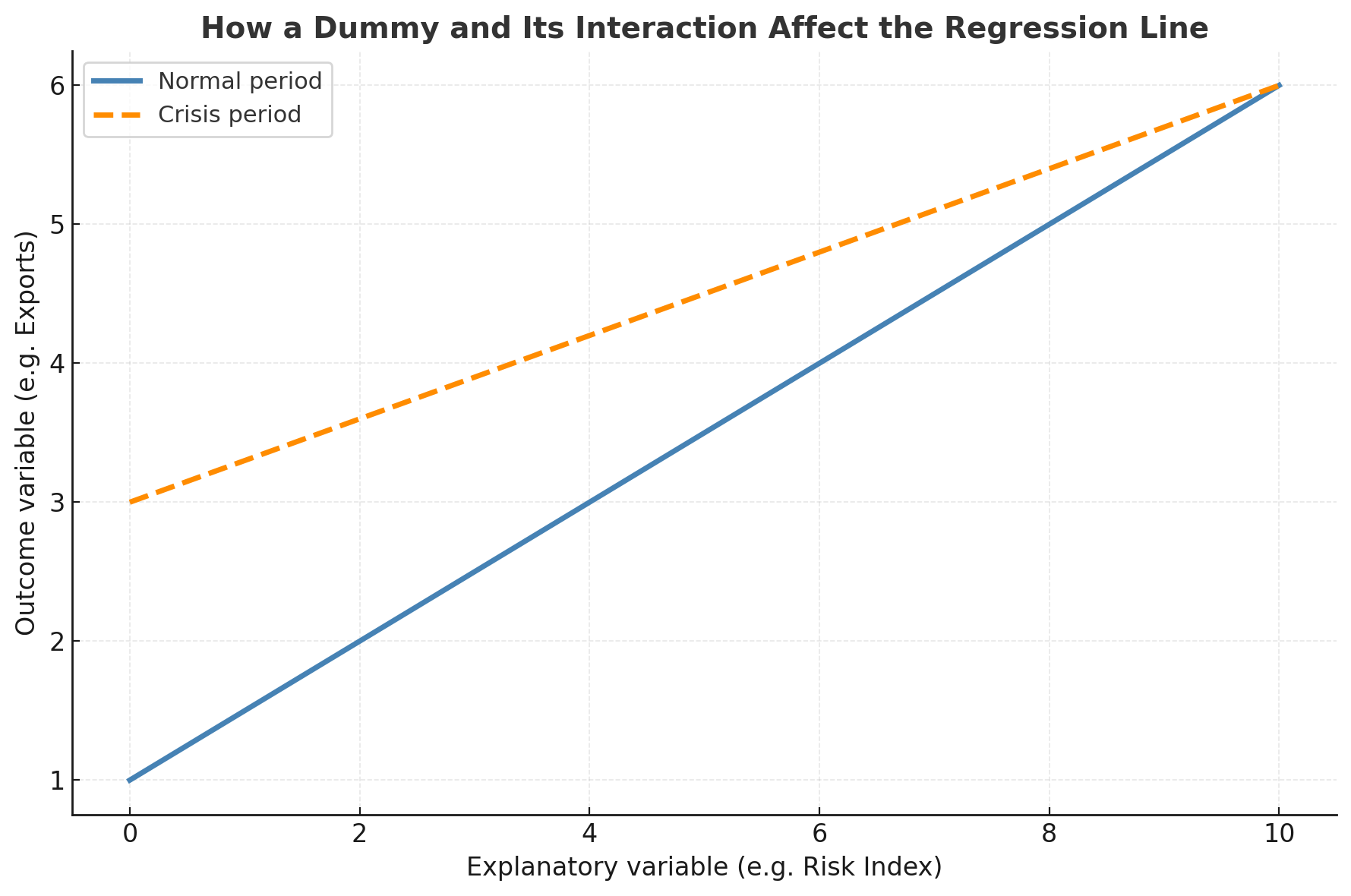
(Normal period: blue solid line. Crisis period: orange dashed line.)
The dummy shifts the intercept vertically, while the interaction modifies the slope. Together they allow the two lines to diverge or converge as X increases. The dummy alone impacts only the starting point, not the slope.
If we omit the dummy and keep only the interaction term, the two lines would be forced to cross at X=0. This would constrain both regimes to share the same intercept, which is rarely realistic in economic data.
Figure 2. Dummy versus Interaction: With and Without Intercept Difference
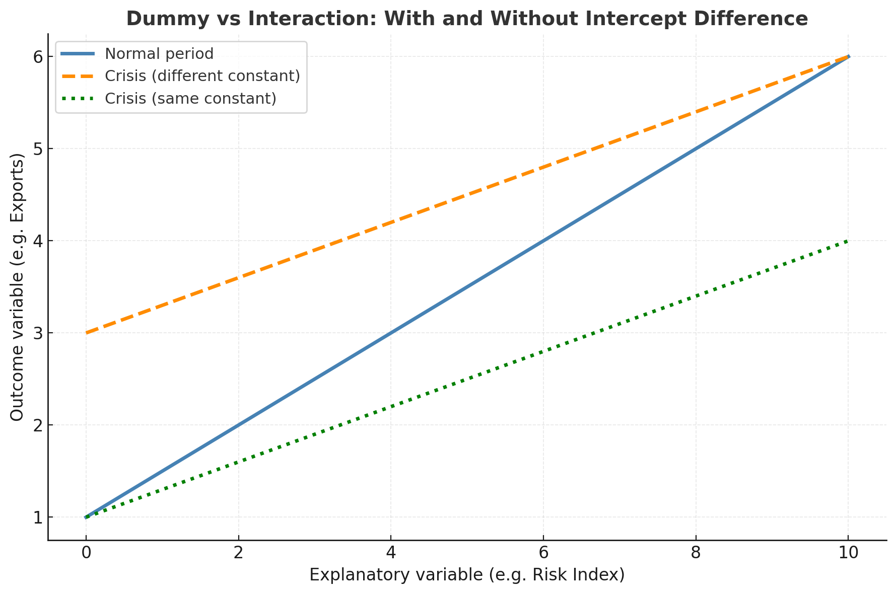
(Normal period: blue solid line. Crisis with different constant: orange dashed line. Crisis with same constant: green dotted line.)
The green line in this second figure illustrates what happens when we exclude the dummy. Both lines start from the same level but differ in slope. The model can no longer represent distinct baselines.
Why this matters
In empirical work, the inclusion of both the dummy and its interaction ensures that the model properly distinguishes level differences from behavioral differences. The dummy gives each group its own intercept, while the interaction reveals how the relationship between X and y changes across regimes.
If we omit the dummy, we mix level and slope effects and risk misinterpreting the results. In short, the dummy term defines the baseline; the interaction term defines the heterogeneity.