After a series of blogs using RATS, allow me to introduce the estimation of Markov-switching models and unit root tests using RATS. We are going to use the example programs and help files provided by Estima. All the files of this blog are available on my GitHub.
The results of the following research will be replicated:
Camacho, Maximo, (2011), Markov-switching models and the unit root hypothesis in real US GDP, Economics Letters, 112, issue 2, p. 161-164.
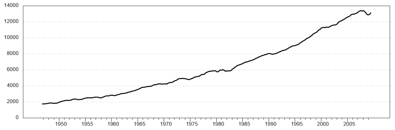
In the following I will start with the model where real US GDP is characterized as trend stationary. Let us look at the data first:
Now, I run the code with latest version of RATS:
*
* Replication file for Camacho(2011), "Markov-switching models and the
* unit root hypothesis in real U.S. GDP", Economics Letters, vol. 112,
* 161-164
*
open data gdp.txt
calendar(q) 1947:1
data(format=prn,nolabels,org=columns) 1947:01 2009:04 date gdp
*
set loggdp = 100.0*log(gdp)
set dlog = loggdp-loggdp{1}
*
* This uses a non-standard trend
*
set trend = 1+.1*(t-1)
*
@MSRegression(switch=c,nfix=2,regimes=2) loggdp
# trend loggdp{1} constant
*
@MSRegParmSet(parmset=regparms)
nonlin(parmset=msparms) p
*
compute gstart=1947:2,gend=2009:4
*
* @MSRegInitial doesn't do very well with this model. It separates the
* two regimes by making the intercept in the first lower than the
* intercept in the second, with the gap set based upon the standard
* error of the intercept in a non-switching regression. However, because
* the AR has a near-unit root, the standard error on the constant (and
* trend) coefficients is extremely high because small changes to the AR
* coefficient create large changes to the deterministics. Instead, this
* does the linear regression, then restricts the AR coefficient to be
* exactly the estimate---this removes that source of uncertainty and
* thus gets the separation to a more reasonable distance.
*
linreg loggdp
# trend loggdp{1} constant
restrict(replace,create) 1
# 2
# 1.0 %beta(2)
*
compute sigsq=%seesq
compute gammas=||%beta(1),%beta(2)||
compute betas(1)=%beta(3)-.5*%stderrs(3)
compute betas(2)=%beta(3)+.5*%stderrs(3)
*
* High (2nd) regime is more persistent than the low (1st) regime
*
compute p=||.75,.10||
*
frml logl = f=%MSRegFVec(t),fpt=%MSProb(t,f),log(fpt)
@MSFilterInit
maximize(start=%(%MSRegInitVariances(),pstar=%msinit()),$
parmset=regparms+msparms,$
method=bfgs,pmethod=simplex,piters=2) logl gstart gend
*
@MSSmoothed gstart gend psmooth
@NBERCycles(down=recession)
set p1smooth = psmooth(t)(1)
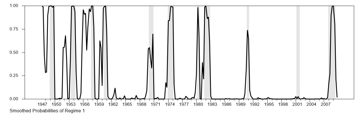
graph(footer="Smoothed Probabilities of Regime 1",max=1.0,min=0.0,$
shading=recession)
# p1smooth gstart gend
*
summarize(title="Average Length of Expansion") 1.0/%beta(7)
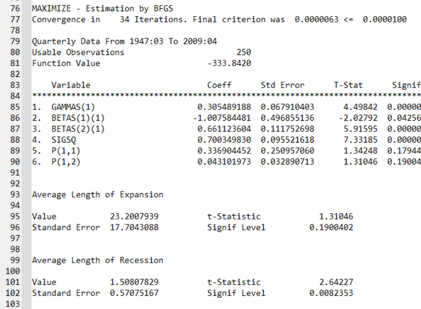
summarize(title="Average Length of Recession") 1.0/(1-%beta(6))We can discuss the results:
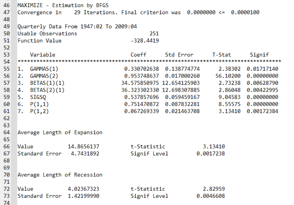
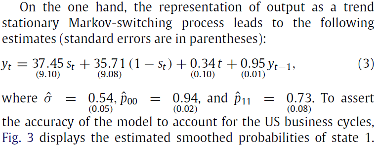
According to these last results, the AR(1) coefficient is around 0.95 (0.01), the trend coefficient is around 0.33 (0.13), constant in state 1 (recession state) is equal to 34.5 (12.65), and constant in state 2 (non-recession state) is equal to 36.32 (12.69). Standard errors in parentheses. The average length of a recession is similar to what we have in the paper.
NBER recessions are quite remarkably reproduced except for the 2001 recession:
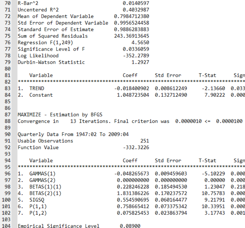
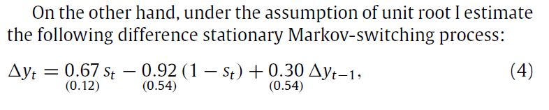
What happens when we restrict the model to have a unit root?
* Restricted model
*
release betas
*
@MSRegression(switch=c,nfix=1,regimes=2) dlog
# dlog{1} constant
compute gstart=1947:3,gend=2009:4
@MSRegParmset(parmset=regparms)
nonlin(parmset=msparms) p
@MSRegInitial gstart gend
@MSFilterInit
compute p=||.75,.10||
maximize(start=%(%MSRegInitVariances(),pstar=%msinit()),$
parmset=regparms+msparms,$
method=bfgs,pmethod=simplex,piters=2) logl gstart gend
*
@MSSmoothed gstart gend psmooth
@NBERCycles(down=recession)
set p1smooth = psmooth(t)(1)
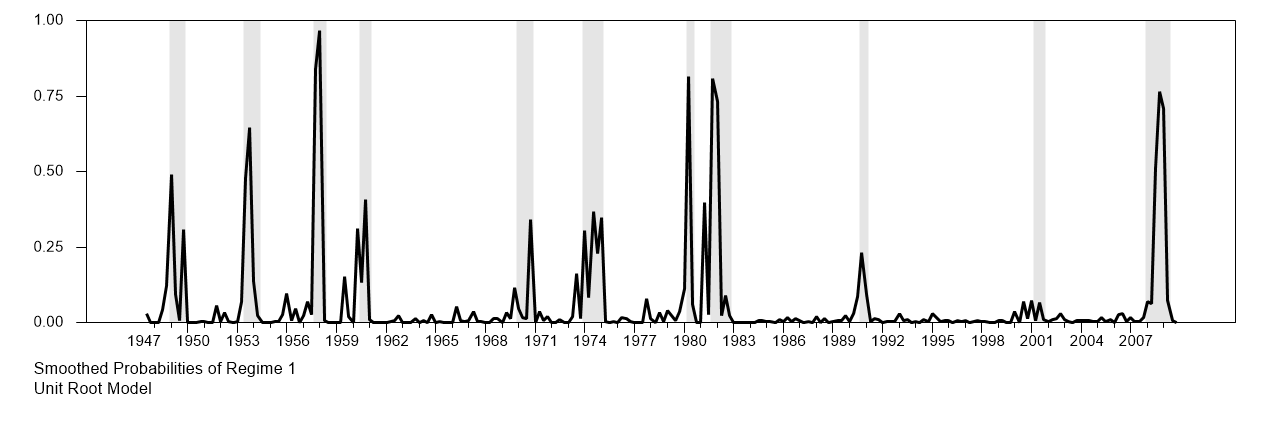
graph(footer="Smoothed Probabilities of Regime 1\\Unit Root Model",max=1.0,min=0.0,$
shading=recession)
# p1smooth gstart gend
summarize(title="Average Length of Expansion") 1.0/%beta(6)
summarize(title="Average Length of Recession") 1.0/(1-%beta(5))
*
Again, the results are roughly reproduced, note that we do not have to estimate the AR(1) coefficient anymore has we imposed the unit-root on US GDP.
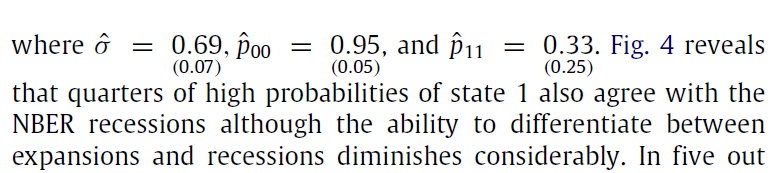
NBER recessions are less predicted now. It is more difficult to distinguish between recessions and non-recession states:
We can also make a unit root test based on the MS model with 1000 draws:
*
* Replication file for Camacho, "Markov-switching models and the unit
* root hypothesis in real U.S. GDP", Economics Letters, vol. 112, 161-164
*
open data gdp.txt
calendar(q) 1947:1
data(format=prn,nolabels,org=columns) 1947:01 2009:04 date gdp
*
set loggdp = 100.0*log(gdp)
set dlog   = loggdp-loggdp{1}
*
* This uses a non-standard trend
*
set trend = 1+.1*(t-1)
*
* It's simpler to run the simulations when we use a different series
* name, so we can replace it with simulated data easily.
*
set logy  = loggdp
set dlogy = dlog
*
@MSRegression(switch=c,nfix=2,regimes=2) dlogy
# trend logy{1} constant
*
@MSRegParmset(parmset=regparms)
nonlin(parmset=msparms)  p
*
compute gstart=1947:2,gend=2009:4
*
* @MSRegInitial doesn't do very well with this model. It separates the
* two regimes by making the intercept in the first lower than the
* intercept in the second, with the gap set based upon the standard
* error of the intercept in a non-switching regression. However, because
* the AR has a near-unit root, the standard error on the constant (and
* trend) coefficients is extremely high because small changes to the AR
* coefficient create large changes to the deterministics. Instead, this
* does the linear regression, then restricts the AR coefficient to be
* exactly the estimate---this removes that source of uncertainty and
* thus gets the separation to a more reasonable distance.
*
linreg dlogy
# trend logy{1} constant
restrict(create) 1
# 2
# 1.0 %beta(2)
*
compute sigsq=%seesq
compute gammas=||%beta(1),%beta(2)||
compute betas(1)=%beta(3)-.5*%stderrs(3)
compute betas(2)=%beta(3)+.5*%stderrs(3)
*
* High (2nd) regime is more persistent than the low (1st) regime
*
compute p=||.75,.10||
*
frml logl = f=%MSRegFVec(t),fpt=%MSProb(t,f),log(fpt)
@MSFilterInit
maximize(start=%(%MSRegInitVariances(),pstar=%msinit()),$
  parmset=regparms+msparms,$
  method=bhhh,pmethod=simplex,piters=2) logl gstart gend
compute msurstat=%tstats(4)
*
* Re-estimate the model under the null of a unit root (the paper seems
* to describe this wrong).
*
nonlin(parmset=forcenull) gammas(2)=0.0
*
* This again needs some help with guess values
*
linreg dlogy
# trend constant
compute sigsq=%seesq
compute gammas=||%beta(1),0.0||
compute betas(1)=%beta(2)-.5*%stderrs(2)
compute betas(2)=%beta(2)+.5*%stderrs(2)
*
@MSFilterInit
maximize(start=%(%MSRegInitVariances(),pstar=%msinit()),$
  parmset=regparms+msparms+forcenull,$
  method=bfgs,pmethod=simplex,piters=2) logl gstart gend
*
* Save information for generating data
*
compute psave=%mspexpand(p)
dec vect[vect] betasave(2)
ewise betasave(i)=betas(i)
compute gammasave=gammas
compute sigmasave=sqrt(sigsq)
*
compute ndraws=1000
dec vect simstats(ndraws)
infobox(action=define,progress,lower=1,upper=ndraws) $
   "Simulated UR Statistics"
do draw=1,ndraws
   gset MSRegime gstart gend   = %ranbranch(%mcergodic(psave))
   gset MSRegime gstart+1 gend = %ranbranch(%xcol(psave,MSRegime{1}))
   *
   * This uses the pre-sample value from the actual data
   *
   set logy gstart gend = betasave(MSRegime)(1)+gammasave(1)*trend+$
        (1+gammasave(2))*logy{1}+%ran(sigmasave)
   set dlogy gstart gend = logy-logy{1}
   *
   * YUNI is a copy of the data used internally by the MSRegression routines
   *
   set yuni = dlogy
   *
   * The guess values have to be re-done for each simulated data series
   *
   linreg(noprint) dlogy
   # trend logy{1} constant
   restrict(noprint,create) 1
   # 2
   # 1.0 %beta(2)
   compute sigsq=%seesq
   compute gammas=||%beta(1),%beta(2)||
   compute betas(1)=%beta(3)-.5*%stderrs(3)
   compute betas(2)=%beta(3)+.5*%stderrs(3)
   compute p=||.75,.10||
   *
   maximize(start=%(%MSRegInitVariances(),pstar=%msinit()),$
     parmset=regparms+msparms,$
     method=bfgs,pmethod=simplex,piters=2,noprint) logl gstart gend
   compute simstats(draw)=%tstats(4)
   infobox(current=draw)
end do draw
infobox(action=remove)
sstats(mean) 1 ndraws simstats(t)>msurstat>>pvalue
disp "Empirical Significance Level" pvalue
We marginally reject the null of unit root as the p-value is around 9 percent: