After two blogs on SVAR with RATS and on SVAR with sign restrictions with Stata, allow me to introduce the estimation of SVAR with sign restrictions using RATS and Monte Carlo integration. We are going to use the example programs and help files provided by Estima. All the files of this blog are available on my GitHub.
The results of the following research will be replicated:
Farrant, Katie and Peersman, Gert, (2006), Is the Exchange Rate a Shock Absorber or a Source of Shocks? New Empirical Evidence, Journal of Money, Credit and Banking, 38, issue 4, p. 939-961.
In the following I will focus on the case of Japan and the 3-variable model to make this blog short. The first part of the code is quite usual for the 3-variable model. You need to localize the routine on your computer called “mcsignrestrict.src“:
*
* Farrant and Peersman(2006), "Is the Exchange Rate a Shock Absorber or a Source
* of Shocks? New Empirical Evidence", JMCB, vol 38, no. 4, pp 939-961.
*
* Sign restrictions with 3 variable model
*
open data "datasetfp.xlsx"
calendar(q) 1961:1
data(format=xlsx,org=columns) 1961:01 2003:02 yus yemu yuk yjp yca cpus cpemu cpuk cpjp cpca stus stemu $
 stuk stjp stca bxemu bxuk bxjp bxca
*
compute nsteps=29
compute VARDraws=500
*
* y = (real) output, cp = consumer prices, st = interest rate differential,
* bx is bilateral nominal exchange rate (local currency/US$)
*
dec hash[string] longname
compute longname("uk")="United Kingdom"
compute longname("emu")="Euro Area"
compute longname("jp")="Japan"
compute longname("ca")="Canada"
*
source mcsignrestrict.src
*
compute nshocks=3,nvar=3
dec vect[strings] sl(nshocks) vl(nvar)
*compute sl=||"Supply","Demand","Nominal"||
compute sl=||"Supply","Demand"||
compute vl=||"Y-Y*","P-P*","Q"||
*In bold, changed form initially released code.
Then, I will choose the sign restrictions based on the theory of Clarida and Gali (1994):
Clarida, Richard and Galí, Jordi, (1994), Sources of real exchange-rate fluctuations: How important are nominal shocks?, Carnegie-Rochester Conference Series on Public Policy, 41, issue 1, p. 1-56.
*
* Where signs are restricted, it's from steps 1 to 4 (counting 1 as the impact)
* for the output growth differential and prices and just the impact for the real
* exchange rate
*
dec SignDesc SupplyDesc(2)
compute SupplyDesc(1)=||+1,1,4||
compute SupplyDesc(2)=||-2,1,4||
dec SignDesc DemandDesc(3)
compute DemandDesc(1)=||+1,1,4||
compute DemandDesc(2)=||+2,1,4||
compute DemandDesc(3)=||-3,1,1||
dec SignDesc NominalDesc(3)
compute NominalDesc(1)=||+1,1,4||
compute NominalDesc(2)=||+2,1,4||
compute NominalDesc(3)=||+3,1,1||
*
*compute [vect[SignDesc]] SignConstraints=||SupplyDesc,DemandDesc,NominalDesc||
compute [vect[SignDesc]] SignConstraints=||SupplyDesc,DemandDesc||
*
********************************************************************************
The number in bold indicates that the supply shock has, in theory, positive effects on the GDP (the first variable in the system) during the first four quarters (+1). It also has negative effects, in theory, on prices (the second variable in the system) during the first four quarters (-2).
Besides, the demand shock will have a positive effect on the GDP (+1) and a positive effect on prices (+1) during the first four quarters. This time, we also have a restriction on the third variable of the system, the real exchange rate. The demand shock will negatively impact the real exchange rate (-3).
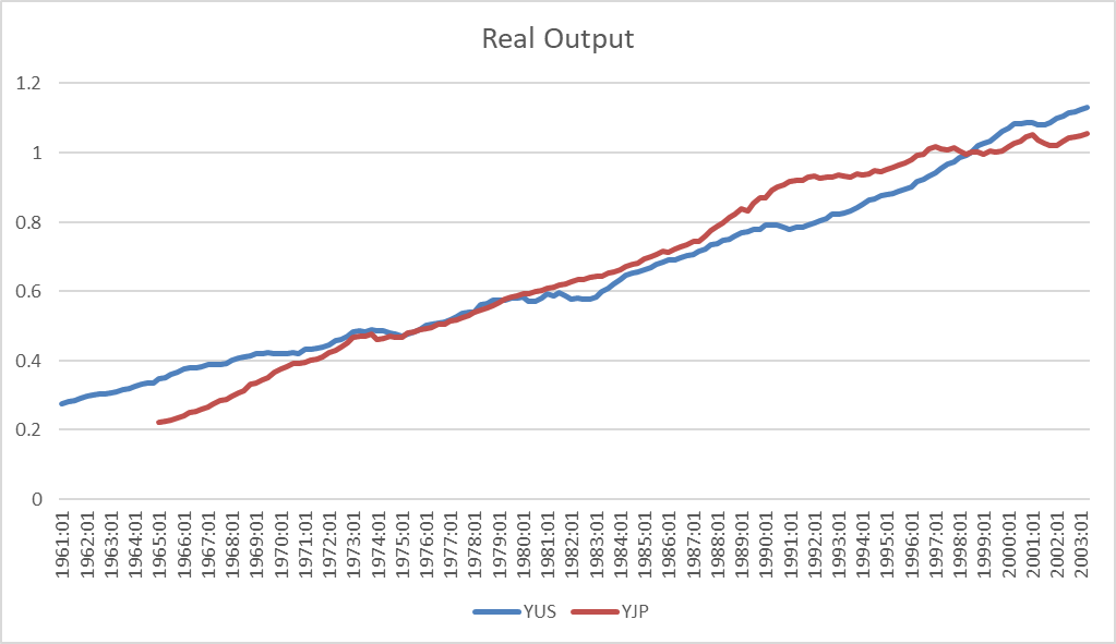
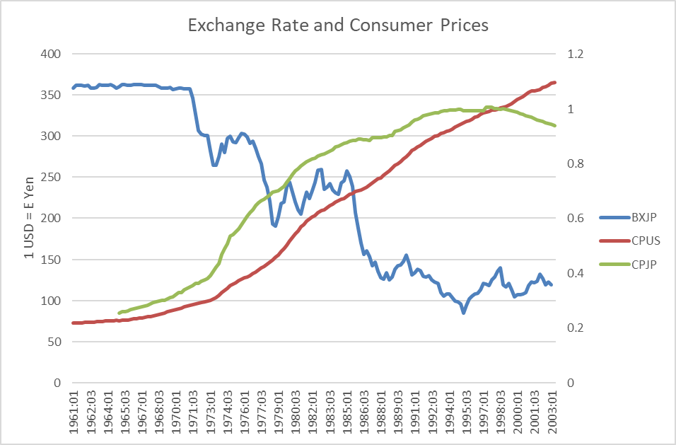
Let us focus on the case of Japan. Using the Excel file, I reproduce the series for Japan:
If you want to run the loop for the other countries, use "uk" "emu" "jp" "ca" instead of "jp":
*
*
dofor [string] zone = "jp"
*"uk" "emu" "jp" "ca"
*
* For each zone, compute
* 100*log ratio of prices vs US
* 100*log real exchange rate
* 100*log ratio of output vs US
*
set lp = 100.0*(log(%s("cp"+zone))-log(cpus))
set lrx = 100.0*log(%s("bx"+zone))-lp
set ly = 100.0*(log(%s("y"+zone))-log(yus))
set dp = lp-lp{1}
set drx = lrx-lrx{1}
set dy = ly-ly{1}
@varlagselect(lags=8,crit=aic,model=var3) 1974:1 2002:4
# dy dp drx
estimate(model=var3) 1974:1 2002:4
@MCSignRestrict(model=var3,nsteps=nsteps,constraints=SignConstraints,$
accum=||1,2,3||,vardraws=VARDraws)
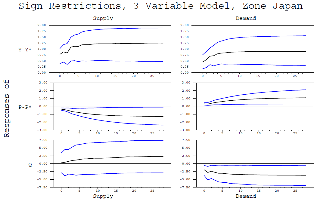
@MCGraphIRF(model=var3,shocklabels=sl,varlabels=vl,$
header="Sign Restrictions, 3 Variable Model, Zone "+longname(zone),picture="##.##",center=median)
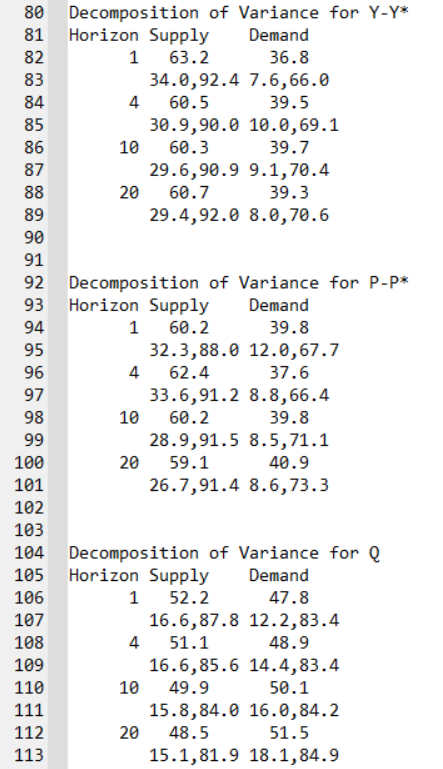
@MCFEVDTable(model=var3,shocklabels=sl,varlabels=vl,horizons=||1,4,10,20||,stddev=1.0)
end dofor
*In bold, changed form initially released code.The confidence intervals are 68 percent bands. The real exchange rate is defined as R= (eP*)/P, so that a decrease in R is termed appreciation of the real exchange rate, an increase is termed depreciation.
We also have the variance decomposition with the 1 standard-deviation confidence intervals: