In this blog, I will show how to estimate Panel VAR with the new command xtvar introduced in StataNow.
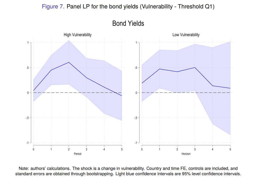
The dataset comes from a paper of mine on the Impact of Climate Risk on Fiscal Space. The Panel Local Projections estimates for the highly vulnerable group give the following results, see my previous blog on that topic:
Let us start with the estimation of the Panel VAR for the highly vulnerable group:
set scheme stcolor

xtdescribe

xtvar bonds_tw Dvul100 ///
 if vul>.3722011, ///
 lags(2) maxldep(2) ///
fd collapse 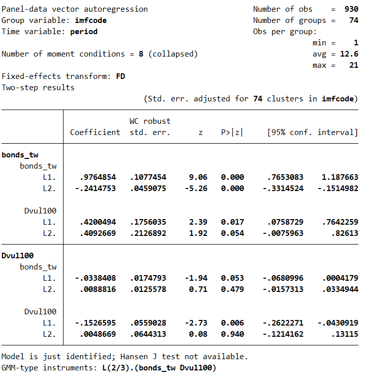
The model is just identified (8 instruments for 8 parameters) and we can test whether the VAR is stable. Besides, we can examine the Granger-causality:
varstable, ///
 graph name(stable, replace)

vargranger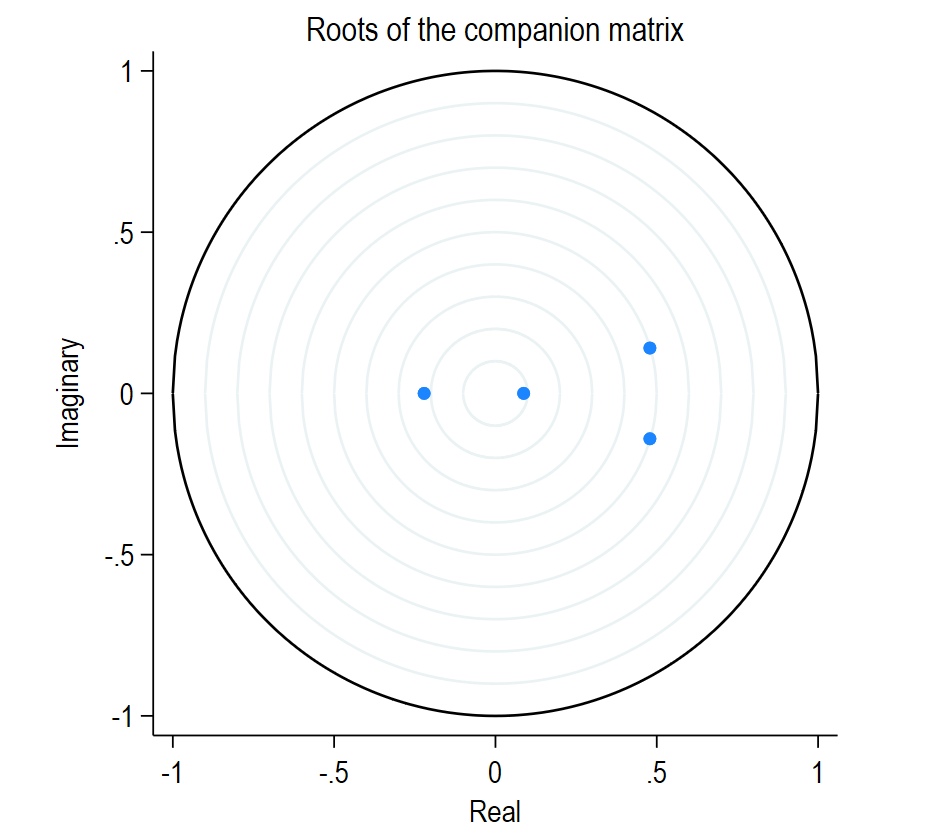
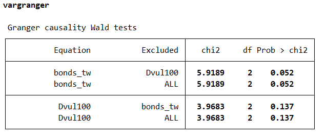
The Granger-causality runs from the vulnerability shocks (Dvul100) towards the bond yields (bonds_tw), since the p-values are below 10 percent in the upper panels.
We can plot the impulse response functions (IRF), after creating a dataset for the IRF:
irf create lags, ///
 set(example1) step(6) replace

irf graph irf, irf(lags) ///
 name(irf, replace)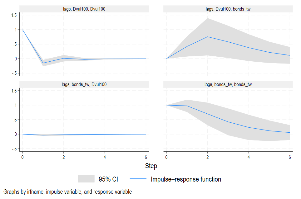
Finally, I can plot the orthogonalized impulse response functions (equivalent to the previous figure in a bivariate Panel VAR):
irf cgraph ///
  (lags Dvul100 bonds_tw irf) ///
  (lags bonds_tw Dvul100 irf), ///
  ycommon name(oirf, replace)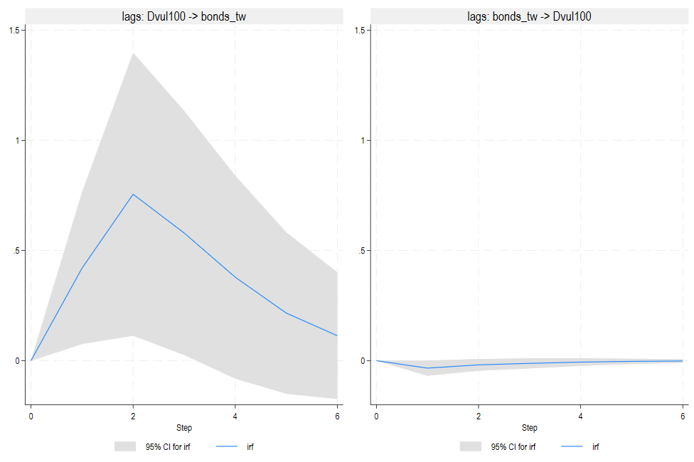
As in the Local Projections estimates, a unit-increase in vulnerability causes an increase in bond yields between 0.5 and 1 percent.