In my previous blog, I recall that we can demonstrate in a few steps that the sample variance is an unbiased estimator of the population variance when we divide by n-1:
\begin{aligned}
E(S^2)&=E\Big[\frac{\Sigma_{i=1}^n (X_i-\bar X)^2}{n-1}\Big]\\
&=\sigma^2
\end{aligned}
Another way to think about this problem is to illustrate the bias when the sample variance is divided by just n. In this blog, I will use the new Wolfram function AIAssistant, that I discussed in another more recent blog, to illustrate the sample variance bias in R and in Mathematica.
So let us start with asking to write an example in R, I asked:
show me a graph of the sample variance bias in RThe answer:
set.seed(123) # for reproducibility
n <- 10 # sample size
N <- 1000 # number of simulations
true_variance <- 1 # true population variance
# create a function to simulate the bias in the sample variance estimator
sample_variance_bias <- function() {
x <- rnorm(n, mean = 0, sd = sqrt(true_variance)) # generate a sample from a normal distribution
biased_estimator <- sum((x - mean(x))^2) / n # compute the biased estimator (dividing by n instead of n-1)
unbiased_estimator <- sum((x - mean(x))^2) / (n - 1) # compute the unbiased estimator (dividing by n-1)
return(biased_estimator - true_variance) # return the bias of the biased estimator
}
# simulate the bias across N simulations
bias <- replicate(N, sample_variance_bias())
# plot the histogram of the bias
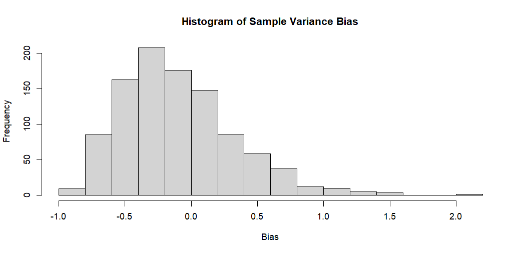
hist(bias, main = "Histogram of Sample Variance Bias", xlab = "Bias", ylab = "Frequency")The description of that code is also provided:
This code generates a sample of size n from a normal distribution with mean 0 and standard deviation equal to the square root of the true population variance. It then computes both the biased estimator (dividing by n instead of n-1) and the unbiased estimator (dividing by n-1). This process is repeated across N simulations, and the bias of the biased estimator is computed for each simulation. Finally, a histogram of the bias values is plotted.

The resulting histogram should show a peak at a negative value, indicating that the biased estimator tends to underestimate the true variance of the population.
The result is pretty neat. We clearly see the downward bias for the sample variance bias estimator. Besides, the explanation is very clear.
By curiosity, I wanted to know whether this R code could be translated into the Wolfram Language.
write me the equivalent for MathematicaThe answer:
SeedRandom[123]; (* for reproducibility *)

n = 10; (* sample size *)
N = 1000; (* number of simulations *)

trueVariance = 1; (* true population variance *)

(* define a function to simulate the bias in the sample variance \
estimator *)
sampleVarianceBias[] := Module[{x, biasedEstimator, unbiasedEstimator},
    x = RandomVariate[NormalDistribution[0, Sqrt[trueVariance]], n]; (*
  generate a sample from a normal distribution *)
    biasedEstimator = Total[(x - Mean[x])^2]/n; (*
  compute the biased estimator (dividing by n instead of n-1) *)
    unbiasedEstimator = Total[(x - Mean[x])^2]/(n - 1); (*
  compute the unbiased estimator (dividing by n-1) *)
    biasedEstimator - trueVariance (*
  return the bias of the biased estimator *)
  ]

(* simulate the bias across N simulations *)
bias = Table[sampleVarianceBias[], N];

(* plot the histogram of the bias *)
Histogram[bias, Automatic, "PDF",
   PlotLabel -> "Histogram of Sample Variance Bias",
   AxesLabel -> {"Bias", "Frequency"}]
This code does not work as the N symbol is protected in Mathematica, so I entered the first error message:
"Symbol N is Protected."The answer:
The error message you are seeing is "Symbol N is Protected". This means that you cannot assign a value to the symbol N because it is already defined as a protected symbol in Mathematica. A protected symbol is one that has special meaning or functionality in the language and cannot be modified by the user.

To fix this error, you can simply use a different symbol name for the number of simulations, such as numSims or simNum. For example:
SeedRandom[123]; (* for reproducibility *)
n = 10; (* sample size *)
numSims = 1000; (* number of simulations *)
trueVariance = 1; (* true population variance *)
(* define a function to simulate the bias in the sample variance \
estimator *)
sampleVarianceBias[] := Module[{x, biasedEstimator, unbiasedEstimator},
x = RandomVariate[NormalDistribution[0, Sqrt[trueVariance]], n]; (*
generate a sample from a normal distribution *)
biasedEstimator = Total[(x - Mean[x])^2]/n; (*
compute the biased estimator (dividing by n instead of n-1) *)
unbiasedEstimator = Total[(x - Mean[x])^2]/(n - 1); (*
compute the unbiased estimator (dividing by n-1) *)
biasedEstimator - trueVariance (*
return the bias of the biased estimator *)
]
(* simulate the bias across numSims simulations *)
bias = Table[sampleVarianceBias[], numSims];
(* plot the histogram of the bias *)
Histogram[bias, Automatic, "Count",
PlotLabel -> "Histogram of Sample Variance Bias",
AxesLabel -> {"Bias", "Frequency"},
PlotRange -> {{-1, 2}, {0, 150}}, ChartStyle -> "Pastel",
ImageSize -> {800, 400}]This code should run without errors and produce the expected histogram.The result, after changing a bit of the Histogram command:

We clearly see that using n in the sample variance formula produces a bias, as the distribution does not peak at 0.
Please note that the files for replicating this blog are available here: https://github.com/JamelSaadaoui/EconMacroBlog
1 Comment
[…] this other blog, I used the new Wolfram function AIAssistant to illustrate the sample variance bias in R and in […]