Drawing Maps for the Largest Cities in the World with Geoplot

Today, we will see how to draw maps with Stata for the largest cities in the world. I used geoplot with multiple frames and an orthographic projection. I recommand to read my previous blog on a similar topic (available here on EconMacro).

Key takeaways:

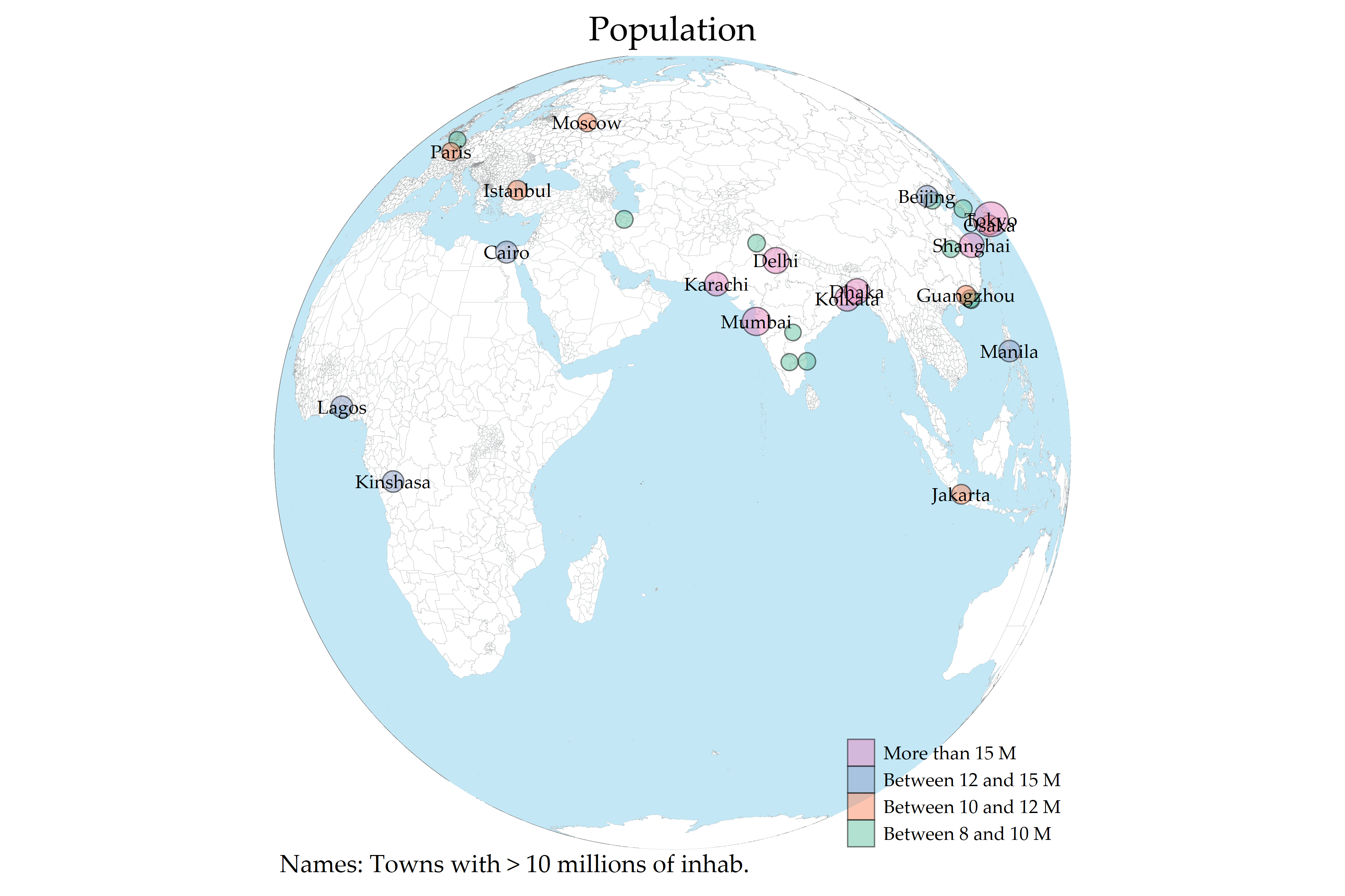
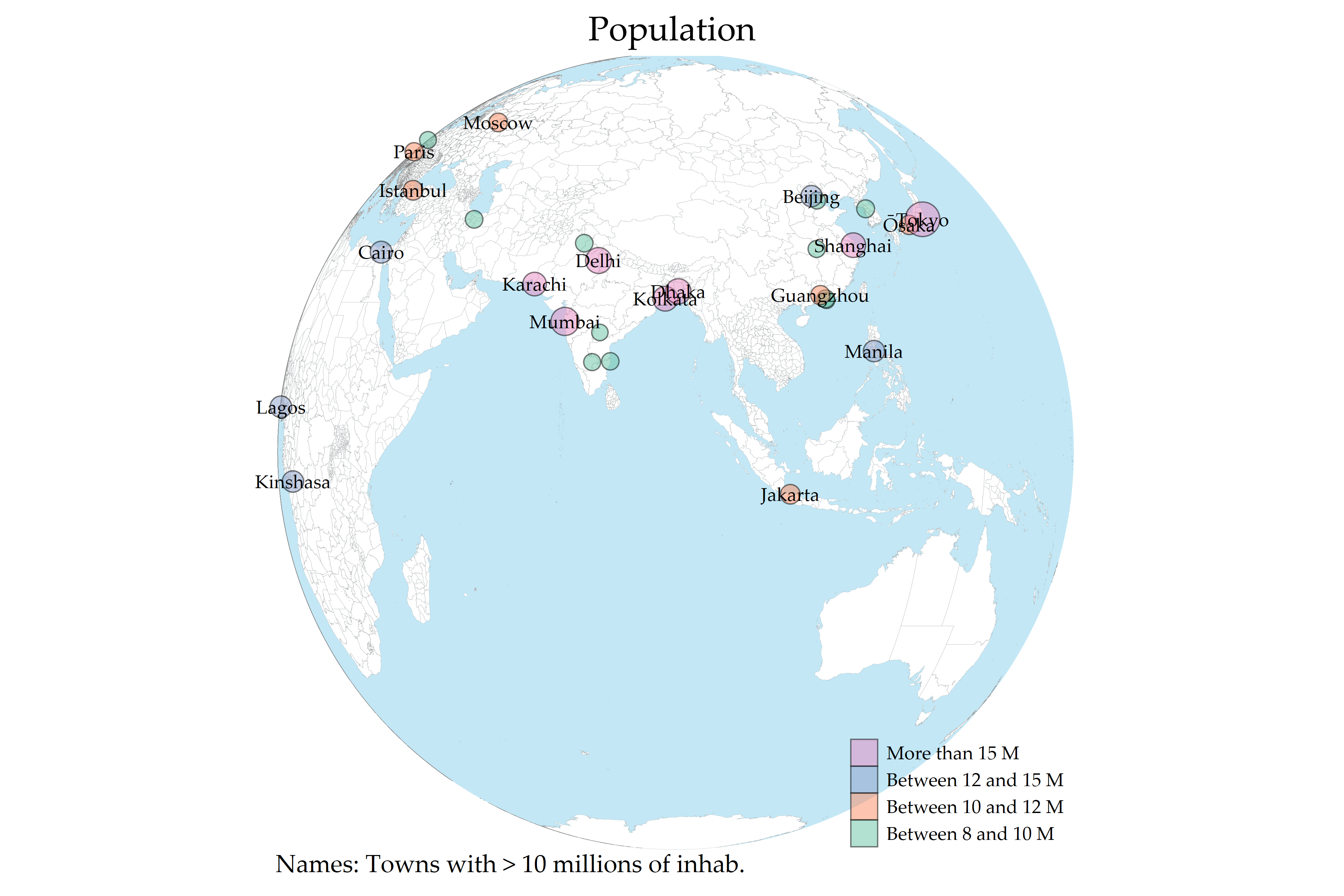
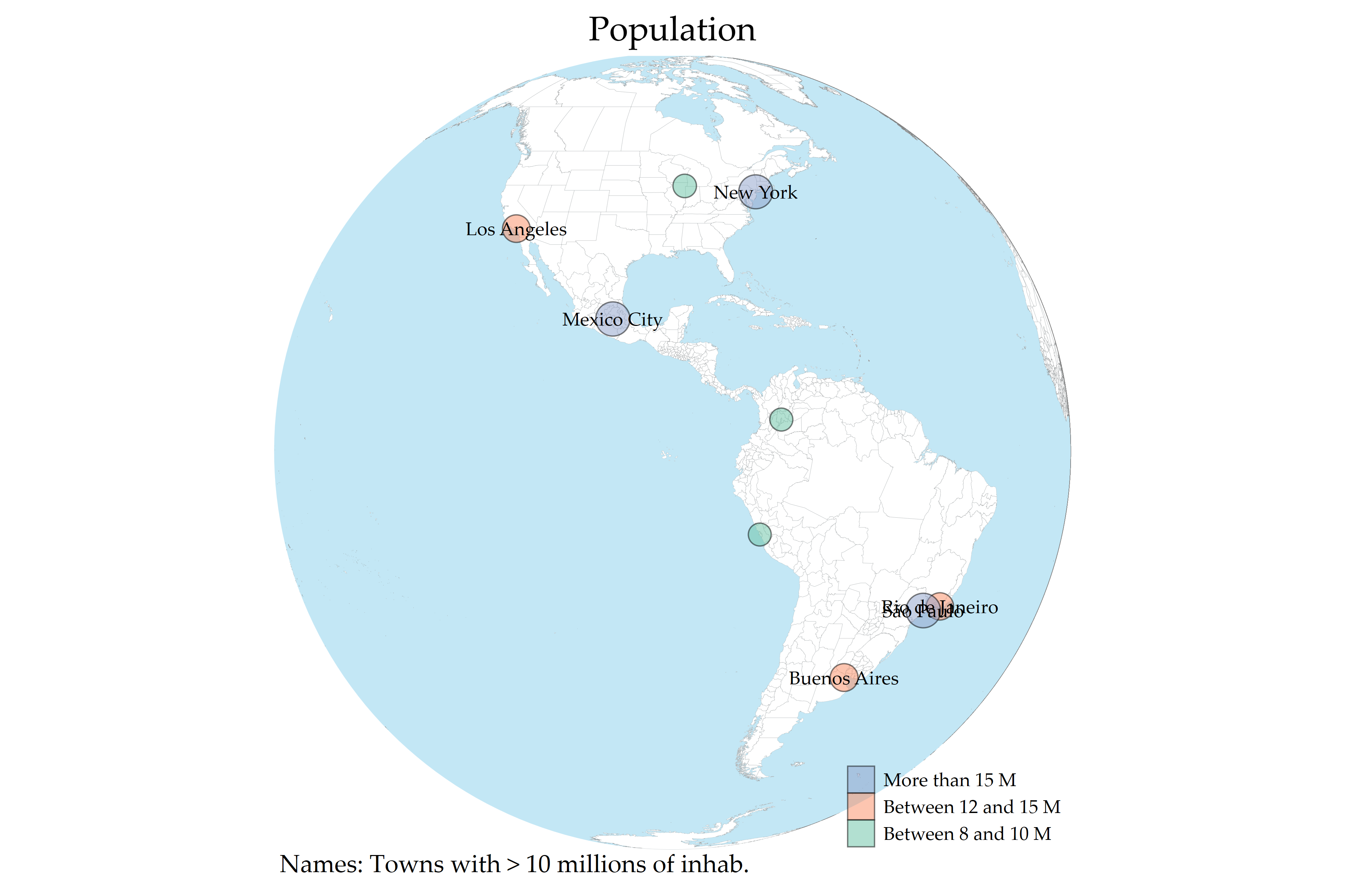
Earth is a sphere, the orthographic projection (more on that here on Wikipedia) gives a better sense of that;
Ben Jann’s geoplot is very versatile for overlapping multiple layers in maps with Stata;
Do not forget to clear the frames before running the full code, it may create problems;
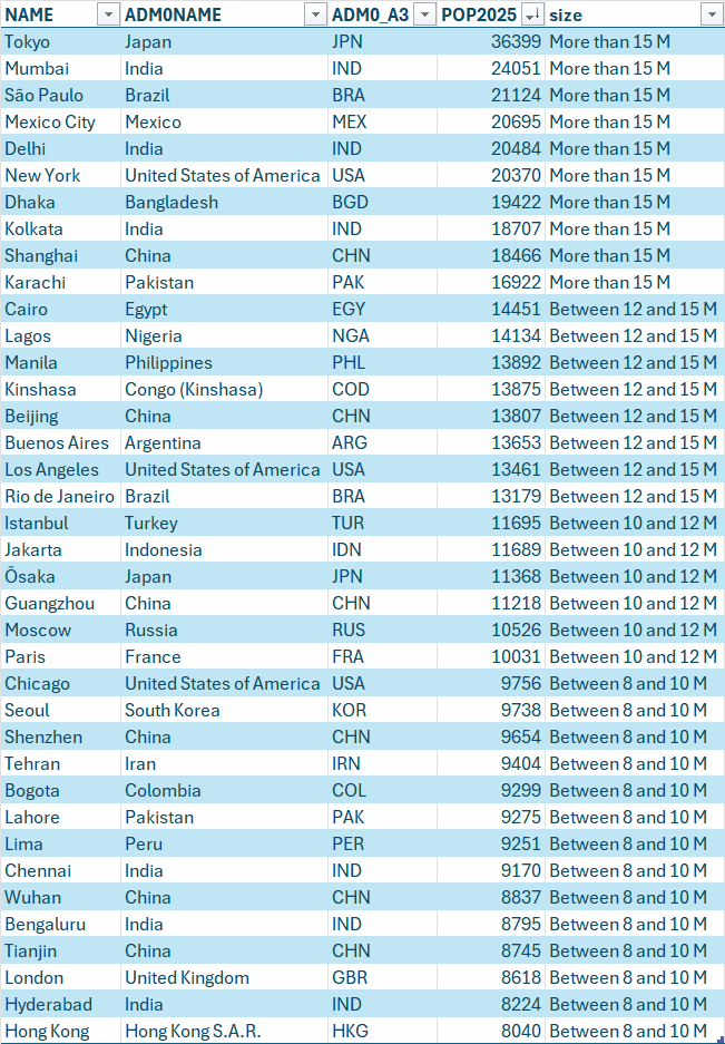
South Asia has 9 large cities (more than 8 million inhabitants, urban population), Africa has 3 large cities, Europe has 4 large cities (including Istanbul and Moscow…), East Asia has 11 large cities (Tokyo being the largest), the Americas have 9 large cities.

The country list is given below:

Full code is explained below, and the update is available on my GitHub (use the ne_10m_populated_places_aug25_world.do):

**# Download the map files

clear
clear frames

/*

https://www.naturalearthdata.com/http//www.naturalearthdata.com/download/10m/cultural/ne_10m_populated_places.zip

*/

spshape2dta data\ne_10m_populated_places, replace

// Sort ID in the SHP file

use ne_10m_populated_places_shp.dta, replace

/*
https://www.statalist.org/forums/forum/
general-stata-discussion/general/
1583924-very-weird-spmap-problem-master-data-not-sorted
*/

sort _ID

save ne_10m_populated_places_shp.dta, replace

use ne_10m_populated_places.dta, replace

**# Histogram of Population in 2025

hist POP2025 if POP2025!=0, addlabel frequency ///
 xlabel(0(5000)40000)

drop if POP2025==.
drop if POP2025<=8000

hist POP2025, addlabel frequency ///
 xlabel(8000(4000)40000)

gen size = 0
replace size = 1 if POP2025 > 10000 & POP2025 < 12000  
replace size = 2 if POP2025 > 12000 & POP2025 < 15000
replace size = 3 if POP2025 > 15000 

label define sizeV 0 "Between 8 and 10 M" ///
 1 "Between 10 and 12 M" 2 "Between 12 and 15 M" ///
 3 "More than 15 M"

label values size sizeV

save ne_10m_populated_places_V2.dta, replace  

// Create two geoframes

geoframe create towns ///
 ne_10m_populated_places_V2.dta, id(_ID) ///
 coord(_CX _CY) ///
 replace 
  
geoframe create regions ///
 ne_10m_admin_1_states_provinces.dta, id(_ID) ///
 coord(_CX _CY) ///
 replace

// Draw the map with two layers

geoplot ///
 (area regions, color(white)) ///
 (line regions, lwidth(vvthin)) ///
 (symbol towns (circle) i.size [w=POP2025] ///
 if _CX>-10 & POP2025>=8000, ///
 color(Set2%50) lcolor(black) size(*3)) ///
 (label towns NAME if _CX>-10 & POP2025>10000, ///
 color(black) size(vsmall)) ///
  , ///
  legend(position(se))  ///
  title("Population") ///
  note( ///
  Names: Towns with > 10 millions of inhab.) ///
  project(orthographic 20 60) background(water)
  
graph rename Graph map_world_regions_frame_new, replace
graph export figures\map_world_regions_frame_new.png, as(png) ///
 width(4000) replace
graph export figures\map_world_regions_frame_new.pdf, as(pdf) ///
 replace
 
geoplot ///
 (area regions, color(white)) ///
 (line regions, lwidth(vvthin)) ///
 (symbol towns (circle) i.size [w=POP2025] ///
 if _CX>-10 & POP2025>=8000, ///
 color(Set2%50) lcolor(black) size(*3)) ///
 (label towns NAME if _CX>-10 & POP2025>10000, ///
 color(black) size(vsmall)) ///
  , ///
  legend(position(se))  ///
  title("Population") ///
  note( ///
  Names: Towns with > 10 millions of inhab.) ///
  project(orthographic 50 90) background(water)
  
graph rename Graph map_world_regions_frame_new_V2, replace
graph export figures\map_world_regions_frame_new_V2.png, as(png) ///
 width(4000) replace
graph export figures\map_world_regions_frame_new_V2.pdf, as(pdf) ///
 replace

geoplot ///
 (area regions, color(white)) ///
 (line regions, lwidth(vvthin)) ///
 (symbol towns (circle) i.size [w=POP2025] ///
 if _CX<-10 & POP2025>=8000, ///
 color(Set2%50) lcolor(black) size(*3)) ///
 (label towns NAME if _CX<-10 & POP2025>10000, ///
 color(black) size(vsmall)) ///
  , ///
  legend(position(se))  ///
  title("Population") ///
  note( ///
  Names: Towns with > 10 millions of inhab.) ///
  project(orthographic 1 -90) background(water)
  
graph rename Graph map_world_regions_frame_new_V3, replace
graph export figures\map_world_regions_frame_new_V3.png, as(png) ///
 width(4000) replace
graph export figures\map_world_regions_frame_new_V3.pdf, as(pdf) ///
 replace

frame dir

*frames save myframeset, ///
frames(regions towns regions_shp towns_shp) replace

Conclusion:

As we have seen in this blog, it is possible to draw maps in Stata at the regional level in some simple steps, using orthographic projection (azimuthal). The files for replicating the results in this blog are available on my GitHub.