Before reading this blog, I recommend you to read the first 2 parts of this blog series. Available below:
In Part I, I focused on Figure 3 of Caldara, Conlisk, Iacoviello, and Penn and showed that a pooled panel Bayesian VAR in Stata/Mata can recover the main historical dynamics reported in the paper: after an adverse country-specific geopolitical risk shock, inflation rises, GDP falls, trade contracts, shortages increase, and fiscal-monetary variables move in an expansionary direction.
In Part II, I turned to Figure 4 and showed that the decomposition between geopolitical acts and geopolitical threats also survives replication rather well: both shocks are inflationary and contractionary, but acts are generally stronger and more persistent.
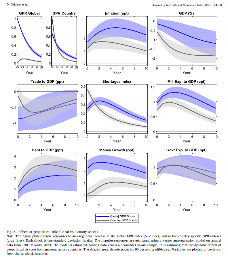
This third post turns to Figure 5, which is, in some sense, the most conceptually subtle figure so far.
The paper no longer asks whether geopolitical risk is inflationary in general, nor whether acts differ from threats. Instead, it asks whether it matters if the shock is global in scope or country-specific.
This is an important distinction. A global shock can move commodity prices, trade routes, and expectations across many economies at once. A country-specific shock, by contrast, may depress local activity more sharply while generating less synchronized international inflationary pressure.
The answer in the paper is clear. Both shocks are inflationary and contractionary, but global shocks appear to generate a stronger inflation response, whereas country-specific shocks are associated with a larger decline in GDP.
That is precisely what makes Figure 5 so interesting. It does not merely restate the baseline result. It refines it by showing that the geographic scope of geopolitical risk matters for macroeconomic transmission.
The replication of Figure 5 turned out to be more delicate than the previous 2 figures.
The difficulty was not really about the broad dynamic patterns. Those were already emerging. The difficult part was scaling.
In Figures 3 and 4, the objects of interest are country-varying series, so the within-country transformation is relatively straightforward. Figure 5 is more subtle because it combines a global GPR index with a country-specific GPR index. That creates an additional normalization problem in the plotted impulse responses, especially for the blue curves associated with the global shock.
In practice, this mattered a lot for the visual replication. At several stages, the global responses were either too small or too large relative to the published figure. The shape was often already correct, but the scale was not.
Once that issue was handled carefully, the figure moved much closer to the one in the paper. That is, in my view, an instructive outcome. It shows that in replication exercises, one can get the economics right before getting the display right. The last mile is often about units, normalization, and graphical comparability rather than about deep econometric disagreement.
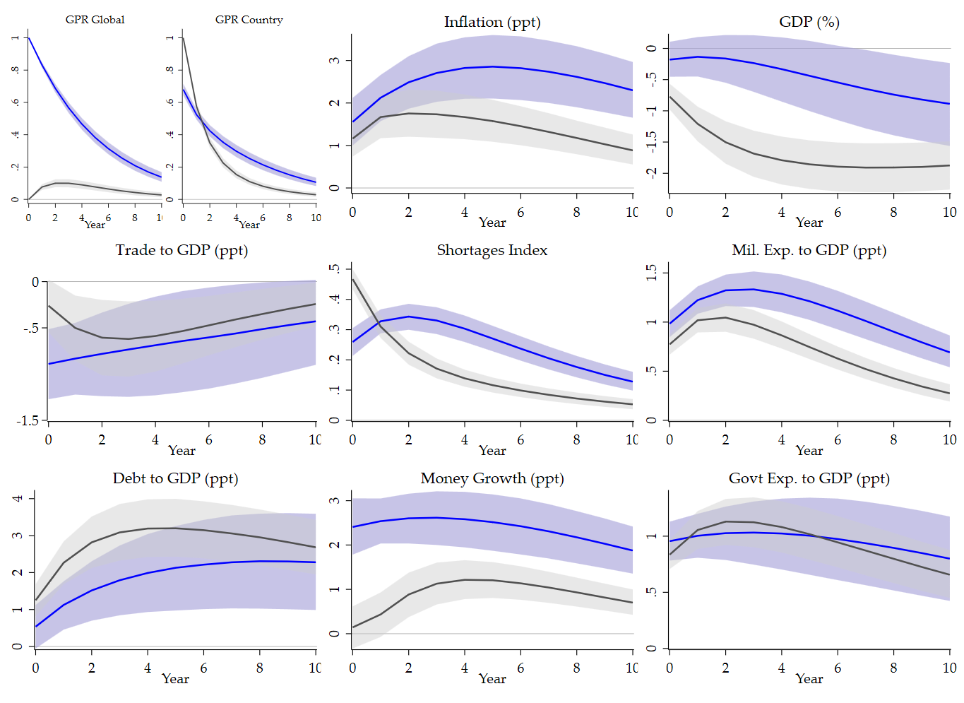
Substantively, the replicated figure confirms the central message of the paper.
Inflation rises after both shocks. But the global shock produces the stronger inflationary response.
GDP falls under both shocks as well, but the contraction is steeper under the country-specific shock.
Trade declines in both cases, and the initial contraction is especially informative because it is consistent with the interpretation that global shocks disrupt international linkages more broadly.
Shortages, military spending, debt, money growth, and government expenditure also move in the expected direction. The general picture is again one of stagflationary pressure, but now with a more refined distinction between worldwide geopolitical disruptions and local geopolitical events.
The 2 small panels on the top left are particularly important. They summarize the identification logic of the figure. The global shock loads on the global GPR index, while the country shock loads on the country GPR index.
That may sound obvious, but it is precisely what must be verified in a good replication. If those panels fail, the rest of the figure becomes harder to interpret. Once those 2 panels look right, the other 8 panels become much more convincing economically.
This is why Figure 5 is more than a robustness check. It tells us something structural. Geopolitical risk is not a single homogeneous macroeconomic object. Its transmission depends on whether the source of the disturbance is broad and synchronized across countries or whether it is concentrated at the country level.
Global shocks appear to be more inflationary. Country-specific shocks are seemingly more contractionary for domestic activity. That is a subtle but important result, and the replication preserves it.
As in the first 2 posts, the right benchmark is not literal code identity with the original implementation. The paper uses a Jeffreys-prior Bayesian VAR with posterior simulation, whereas the replication relies on a custom Stata/Mata workflow designed to reproduce the same empirical object transparently.
Final code
version 18.0

capture log close _f5
log using "$JIE_LOG/22_figure5_global_country.log", replace text ///
    name(_f5)

use "$JIE_DER/annual_panel.dta", clear
sort country_id year
xtset country_id year

local yraw ///
    gpr_global ///
    gpr_country ///
    inflation_ppt ///
    gdp_pct ///
    trade_to_gdp_ppt ///
    shortages_index ///
    milit_exp_to_gdp_ppt ///
    debt_to_gdp_ppt ///
    money_growth_ppt ///
    govt_exp_to_gdp_ppt

egen __rowmiss_f5 = rowmiss(`yraw')
gen byte sample_f5 = (__rowmiss_f5 == 0)
drop __rowmiss_f5

count if sample_f5
display as text "Figure 5 raw complete-case observations: " r(N)

foreach v of local yraw {
    by country_id: egen mean_`v'_f5 = mean(cond(sample_f5, `v', .))
    gen dm_`v'_f5 = cond(sample_f5, `v' - mean_`v'_f5, .)
    drop mean_`v'_f5
}

local ydm
foreach v of local yraw {
    local ydm `ydm' dm_`v'_f5
}

mata: jie_bvar_pooled_summary( ///
    "`ydm'", "country_id", "year", "sample_f5", ///
    $JIE_P, $JIE_H, $JIE_NDRAWS, 1, 1, ///
    "F5G_Q05", "F5G_Q50", "F5G_Q95", ///
    "F5G_MEAN", "F5G_VAR", "F5G_Neff" ///
)

mata: jie_bvar_pooled_summary( ///
    "`ydm'", "country_id", "year", "sample_f5", ///
    $JIE_P, $JIE_H, $JIE_NDRAWS, 2, 2, ///
    "F5C_Q05", "F5C_Q50", "F5C_Q95", ///
    "F5C_MEAN", "F5C_VAR", "F5C_Neff" ///
)

display as text "Figure 5 lag-valid pooled rows: " ///
    %9.0g scalar(F5G_Neff)

local cnG05
local cnG50
local cnG95
local cnC05
local cnC50
local cnC95

foreach v of local yraw {
    local cnG05 `cnG05' global_q05_`v'
    local cnG50 `cnG50' global_q50_`v'
    local cnG95 `cnG95' global_q95_`v'
    local cnC05 `cnC05' country_q05_`v'
    local cnC50 `cnC50' country_q50_`v'
    local cnC95 `cnC95' country_q95_`v'
}

matrix colnames F5G_Q05 = `cnG05'
matrix colnames F5G_Q50 = `cnG50'
matrix colnames F5G_Q95 = `cnG95'
matrix colnames F5C_Q05 = `cnC05'
matrix colnames F5C_Q50 = `cnC50'
matrix colnames F5C_Q95 = `cnC95'

preserve
clear
set obs `= $JIE_H + 1'
gen horizon = _n - 1

svmat double F5G_Q05, names(col)
svmat double F5G_Q50, names(col)
svmat double F5G_Q95, names(col)

svmat double F5C_Q05, names(col)
svmat double F5C_Q50, names(col)
svmat double F5C_Q95, names(col)

*------------------------------------------------------------*
* JIE-style display normalization for the blue IRFs
*------------------------------------------------------------*
scalar lambdaG = 0.68 / global_q50_gpr_country[1]

display as text "Figure 5 global scaling factor = " ///
    %9.4f scalar(lambdaG)

local yscale_blue ///
    gpr_country ///
    inflation_ppt ///
    gdp_pct ///
    trade_to_gdp_ppt ///
    shortages_index ///
    milit_exp_to_gdp_ppt ///
    debt_to_gdp_ppt ///
    money_growth_ppt ///
    govt_exp_to_gdp_ppt

foreach v of local yscale_blue {
    replace global_q05_`v' = global_q05_`v' * scalar(lambdaG)
    replace global_q50_`v' = global_q50_`v' * scalar(lambdaG)
    replace global_q95_`v' = global_q95_`v' * scalar(lambdaG)
}

*------------------------------------------------------------*
* Final cosmetic fix:
* rescale ONLY the gray curve in the GPR Global panel
*------------------------------------------------------------*
quietly summarize country_q50_gpr_global, meanonly
scalar peak_cgpr_global = r(max)
scalar lambdaCG = 0.10 / peak_cgpr_global

display as text "Figure 5 gray GPR-global scaling factor = " ///
    %9.4f scalar(lambdaCG)

replace country_q05_gpr_global = ///
    country_q05_gpr_global * scalar(lambdaCG)
replace country_q50_gpr_global = ///
    country_q50_gpr_global * scalar(lambdaCG)
replace country_q95_gpr_global = ///
    country_q95_gpr_global * scalar(lambdaCG)

* GDP in decimal units -> percent
replace global_q05_gdp_pct  = 100 * global_q05_gdp_pct
replace global_q50_gdp_pct  = 100 * global_q50_gdp_pct
replace global_q95_gdp_pct  = 100 * global_q95_gdp_pct

replace country_q05_gdp_pct = 100 * country_q05_gdp_pct
replace country_q50_gdp_pct = 100 * country_q50_gdp_pct
replace country_q95_gdp_pct = 100 * country_q95_gdp_pct

save "$JIE_DER/fig5_irf.dta", replace
export delimited using "$JIE_DER/fig5_irf.csv", replace

local gtitle_gpr_global           "GPR Global"
local gtitle_gpr_country          "GPR Country"
local gtitle_inflation_ppt        "Inflation (ppt)"
local gtitle_gdp_pct              "GDP (%)"
local gtitle_trade_to_gdp_ppt     "Trade to GDP (ppt)"
local gtitle_shortages_index      "Shortages Index"
local gtitle_milit_exp_to_gdp_ppt "Mil. Exp. to GDP (ppt)"
local gtitle_debt_to_gdp_ppt      "Debt to GDP (ppt)"
local gtitle_money_growth_ppt     "Money Growth (ppt)"
local gtitle_govt_exp_to_gdp_ppt  "Govt Exp. to GDP (ppt)"

local yset_gpr_global ///
    "yscale(range(-0.02 1.05)) ylabel(0 .2 .4 .6 .8 1, nogrid labsize(medsmall))"

local yset_gpr_country ///
    "yscale(range(-0.02 1.05)) ylabel(0 .2 .4 .6 .8 1, nogrid labsize(medsmall))"

local yset_inflation_ppt ///
    "yscale(range(-0.1 3.6)) ylabel(0 1 2 3, nogrid labsize(medsmall))"

local yset_gdp_pct ///
    "yscale(range(-2.2 0.2)) ylabel(-2 -1.5 -1 -.5 0, nogrid labsize(medsmall))"

local yset_trade_to_gdp_ppt ///
    "yscale(range(-1.3 0.2) noextend) ylabel(-1.5 -.5 0, angle(horizontal) nogrid labsize(medsmall))"

local yset_shortages_index ///
    "yscale(range(0 .52)) ylabel(0 .1 .2 .3 .4 .5, nogrid labsize(medsmall))"

local yset_milit_exp_to_gdp_ppt ///
    "yscale(range(0 1.6)) ylabel(0 .5 1 1.5, nogrid labsize(medsmall))"

local yset_debt_to_gdp_ppt ///
    "yscale(range(0 4.2)) ylabel(0 1 2 3 4, nogrid labsize(medsmall))"

local yset_money_growth_ppt ///
    "yscale(range(0 3.2)) ylabel(0 1 2 3, nogrid labsize(medsmall))"

local yset_govt_exp_to_gdp_ppt ///
    "yscale(range(0 1.4)) ylabel(0 .5 1, nogrid labsize(medsmall))"

local linecolG "blue"
local bandcolG "lavender"
local linecolC "gs5"
local bandcolC "gs12"

foreach v of local yraw {
    twoway ///
        rarea global_q05_`v' global_q95_`v' horizon, ///
            color(`bandcolG'%65) ///
            lcolor(`bandcolG'%0) || ///
        rarea country_q05_`v' country_q95_`v' horizon, ///
            color(`bandcolC'%45) ///
            lcolor(`bandcolC'%0) || ///
        line global_q50_`v' horizon, ///
            lcolor(`linecolG') lwidth(medthick) || ///
        line country_q50_`v' horizon, ///
            lcolor(`linecolC') lwidth(medthick) || ///
        , ///
        title("`gtitle_`v''", size(medium) color(black)) ///
        yline(0, lcolor(black%35) lwidth(vthin)) ///
        xtitle("Year", size(medsmall)) ///
        ytitle("") ///
        xlabel(0(2)$JIE_H, labsize(medsmall) nogrid) ///
        `yset_`v'' ///
        legend(off) ///
        graphregion(color(white) margin(small)) ///
        plotregion(color(white) margin(tiny)) ///
        name(gr5_`v', replace)
}

graph combine ///
    gr5_gpr_global ///
    gr5_gpr_country, ///
    cols(2) ///
    imargin(0 0 0 0) ///
    graphregion(color(white) margin(0 0 0 0)) ///
    name(row1_left_f5, replace)

graph combine ///
    row1_left_f5 ///
    gr5_inflation_ppt ///
    gr5_gdp_pct, ///
    cols(3) ///
    imargin(1 1 1 1) ///
    graphregion(color(white) margin(0 0 0 0)) ///
    name(row1_f5, replace)

graph combine ///
    gr5_trade_to_gdp_ppt ///
    gr5_shortages_index ///
    gr5_milit_exp_to_gdp_ppt, ///
    cols(3) ///
    imargin(1 1 1 1) ///
    graphregion(color(white) margin(0 0 0 0)) ///
    name(row2_f5, replace)

graph combine ///
    gr5_debt_to_gdp_ppt ///
    gr5_money_growth_ppt ///
    gr5_govt_exp_to_gdp_ppt, ///
    cols(3) ///
    imargin(1 1 1 1) ///
    graphregion(color(white) margin(0 0 0 0)) ///
    name(row3_f5, replace)

graph combine ///
    row1_f5 ///
    row2_f5 ///
    row3_f5, ///
    cols(1) ///
    imargin(zero) ///
    graphregion(color(white) margin(2 2 2 2)) ///
    name(fig5_combined, replace)

graph save "$JIE_FIG/figure5_global_country_journalstyle.gph", replace
graph export "$JIE_FIG/figure5_global_country_journalstyle.png", ///
    width(2600) replace

restore
log close _f5
Conclusion
A carefully written pooled panel Bayesian VAR in Stata/Mata can recover the same central distinction emphasized in the paper: both global and country-specific geopolitical shocks are inflationary, but global shocks appear to generate stronger inflationary effects, whereas country-specific shocks are associated with a larger contraction in activity.
This is, in my view, an important result. It suggests that geopolitical risk should not be treated as a single homogeneous disturbance. Its macroeconomic consequences depend not only on its intensity, but also on its scope. Once the normalization is handled properly, the figure becomes both visually convincing and economically informative.
References
Caldara, D., Conlisk, S., Iacoviello, M., & Penn, M. (2026). Do geopolitical risks raise or lower inflation? Journal of International Economics, 104188.