Before reading this blog, I recommend you to read the first part of this blog series. Available below:
In Part I, I focused on Figure 3 of Caldara, Conlisk, Iacoviello, and Penn and showed that a pooled panel Bayesian VAR in Stata/Mata can recover the main historical dynamics reported in the paper: after an adverse country-specific geopolitical risk shock, inflation rises, GDP falls, trade contracts, shortages increase, and fiscal-monetary variables move in an expansionary direction. That first exercise was already quite reassuring. It suggested that the core message of the paper is replicable in a meaningful sense.
This follow-up turns to Figure 4, which is even more informative from an economic point of view. Instead of treating geopolitical risk as a single object, the paper decomposes it into 2 components: geopolitical acts and geopolitical threats. The question is simple but important. Do realized adverse events and anticipatory geopolitical tensions transmit differently to inflation, output, trade, shortages, and policy variables? The answer in the paper is yes: both shocks are inflationary and contractionary, but acts are generally larger and more persistent. The figure is estimated on annual data from 1900 through 2023 in the same pooled panel VAR spirit as the baseline analysis.
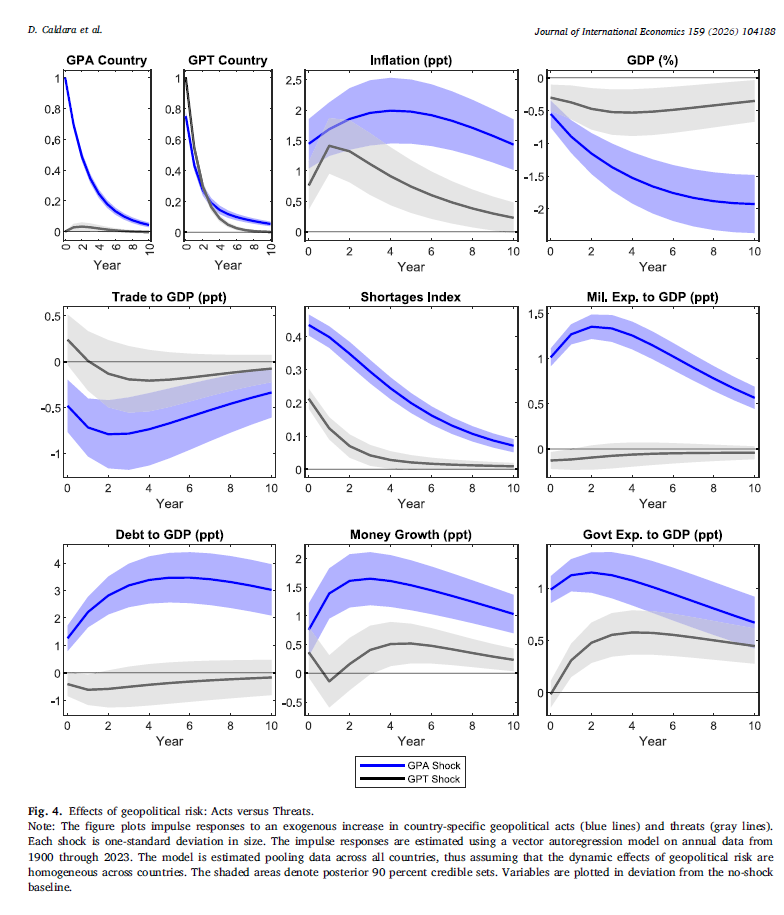
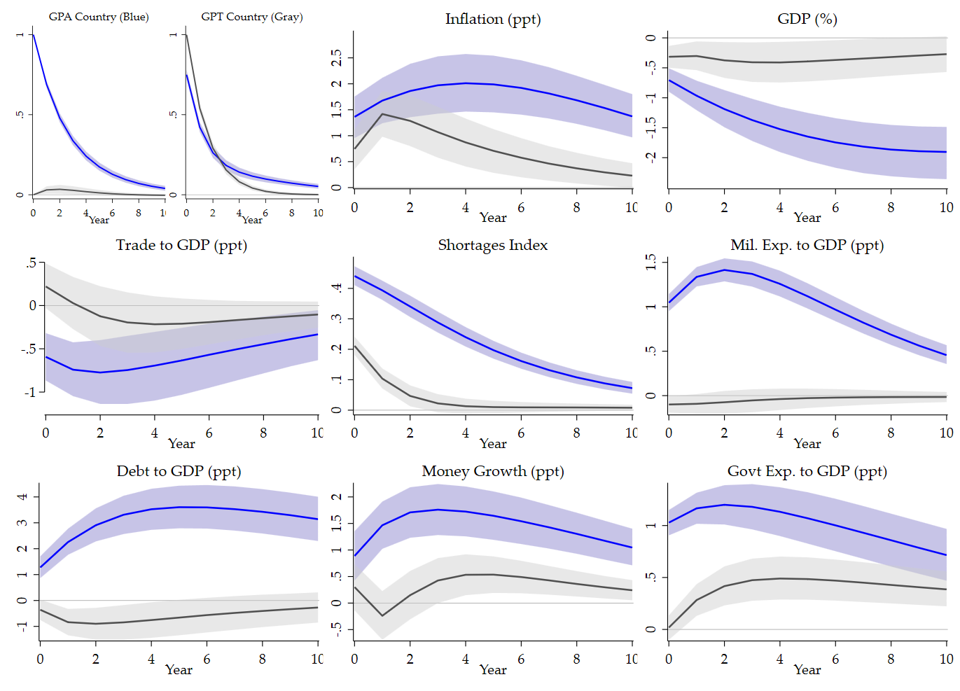
In both versions, geopolitical acts produce a stronger inflation response than geopolitical threats. The blue inflation response is hump-shaped and remains clearly above the gray one over the full horizon. GDP falls after both shocks, but the decline associated with acts is markedly larger. Trade contracts more after acts, shortages remain elevated after both shocks but are clearly stronger for acts, and military spending, debt, money growth, and government expenditure all display a larger response to acts than to threats.
The 2 small panels on the top left are also important. They show the dynamics of the acts and threats indices themselves. In the published figure, the acts shock loads strongly on the acts index and the threats shock loads strongly on the threats index, while cross-effects remain visible. The replication captures that structure rather well. The shapes are not identical, but the decomposition works in the right direction: acts and threats are not the same shock, and the figure makes that distinction economically interpretable.
Substantively, Figure 4 sharpens the main message of Part I. The inflationary consequences of geopolitical risk are not driven only by realized conflict, nor only by perceived risk. Both matter. But realized acts appear to trigger a broader and stronger macroeconomic adjustment. That is consistent with the idea that actual geopolitical events carry more immediate consequences for trade, shortages, fiscal behavior, and macroeconomic expectations than mere threats, even though threats are by no means innocuous. In that sense, Figure 4 is not just a robustness exercise. It tells us something structural about the channels through which geopolitics enters the macroeconomy.
The paper relies on a Jeffreys-prior Bayesian VAR with posterior simulation, while my implementation is a custom pooled panel Bayesian VAR written in Stata/Mata to reproduce the same empirical object in a transparent way. The correct standard is therefore not literal code identity, but whether the replicated figure preserves the signs, shapes, relative magnitudes, and interpretation of the published impulse responses. On that criterion, the exercise works well. That was already the lesson of Part I, and Figure 4 reinforces it.
My practical recommendation for the blog post is therefore straightforward. Show the published figure first, then the replication, and use the comparison to make 3 points. First, the economic ranking of acts versus threats is replicated. Second, the core macroeconomic message survives the translation into custom Stata/Mata code. Third, the remaining discrepancies are mostly graphical and therefore much less worrying than discrepancies in the underlying dynamics. That is precisely the kind of result one wants from a careful replication exercise.
Final code
version 18.0

capture log close _f4
log using "$JIE_LOG/21_figure4_acts_threats.log", replace text ///
    name(_f4)

use "$JIE_DER/annual_panel.dta", clear
sort country_id year
xtset country_id year

local yraw ///
    gpa_country ///
    gpt_country ///
    inflation_ppt ///
    gdp_pct ///
    trade_to_gdp_ppt ///
    shortages_index ///
    milit_exp_to_gdp_ppt ///
    debt_to_gdp_ppt ///
    money_growth_ppt ///
    govt_exp_to_gdp_ppt

egen __rowmiss_f4 = rowmiss(`yraw')
gen byte sample_f4 = (__rowmiss_f4 == 0)
drop __rowmiss_f4

count if sample_f4
display as text "Figure 4 raw complete-case observations: " r(N)

qui levelsof country if sample_f4, local(countries_f4)
local ncountry : word count `countries_f4'
display as text "Figure 4 countries: `ncountry'"

foreach v of local yraw {
    by country_id: egen mean_`v'_f4 = mean(cond(sample_f4, `v', .))
    gen dm_`v'_f4 = cond(sample_f4, `v' - mean_`v'_f4, .)
}

local ydm
foreach v of local yraw {
    local ydm `ydm' dm_`v'_f4
}

mata: jie_bvar_pooled_summary( ///
    "`ydm'", "country_id", "year", "sample_f4", ///
    $JIE_P, $JIE_H, $JIE_NDRAWS, 1, 1, ///
    "F4A_Q05", "F4A_Q50", "F4A_Q95", ///
    "F4A_MEAN", "F4A_VAR", "F4A_Neff" ///
)

mata: jie_bvar_pooled_summary( ///
    "`ydm'", "country_id", "year", "sample_f4", ///
    $JIE_P, $JIE_H, $JIE_NDRAWS, 2, 2, ///
    "F4T_Q05", "F4T_Q50", "F4T_Q95", ///
    "F4T_MEAN", "F4T_VAR", "F4T_Neff" ///
)

display as text "Figure 4 lag-valid pooled rows (acts): " ///
    %9.0g scalar(F4A_Neff)

display as text "Figure 4 lag-valid pooled rows (threats): " ///
    %9.0g scalar(F4T_Neff)

local cnA05
local cnA50
local cnA95
local cnT05
local cnT50
local cnT95

foreach v of local yraw {
    local cnA05 `cnA05' acts_q05_`v'
    local cnA50 `cnA50' acts_q50_`v'
    local cnA95 `cnA95' acts_q95_`v'
    local cnT05 `cnT05' threats_q05_`v'
    local cnT50 `cnT50' threats_q50_`v'
    local cnT95 `cnT95' threats_q95_`v'
}

matrix colnames F4A_Q05 = `cnA05'
matrix colnames F4A_Q50 = `cnA50'
matrix colnames F4A_Q95 = `cnA95'
matrix colnames F4T_Q05 = `cnT05'
matrix colnames F4T_Q50 = `cnT50'
matrix colnames F4T_Q95 = `cnT95'

preserve
clear
set obs `= $JIE_H + 1'
gen horizon = _n - 1

svmat double F4A_Q05, names(col)
svmat double F4A_Q50, names(col)
svmat double F4A_Q95, names(col)

svmat double F4T_Q05, names(col)
svmat double F4T_Q50, names(col)
svmat double F4T_Q95, names(col)

replace acts_q05_gdp_pct    = 100 * acts_q05_gdp_pct
replace acts_q50_gdp_pct    = 100 * acts_q50_gdp_pct
replace acts_q95_gdp_pct    = 100 * acts_q95_gdp_pct

replace threats_q05_gdp_pct = 100 * threats_q05_gdp_pct
replace threats_q50_gdp_pct = 100 * threats_q50_gdp_pct
replace threats_q95_gdp_pct = 100 * threats_q95_gdp_pct

save "$JIE_DER/fig4_irf.dta", replace
export delimited using "$JIE_DER/fig4_irf.csv", replace

local gtitle_gpa_country          "GPA Country (Blue)"
local gtitle_gpt_country          "GPT Country (Gray)"
local gtitle_inflation_ppt        "Inflation (ppt)"
local gtitle_gdp_pct              "GDP (%)"
local gtitle_trade_to_gdp_ppt     "Trade to GDP (ppt)"
local gtitle_shortages_index      "Shortages Index"
local gtitle_milit_exp_to_gdp_ppt "Mil. Exp. to GDP (ppt)"
local gtitle_debt_to_gdp_ppt      "Debt to GDP (ppt)"
local gtitle_money_growth_ppt     "Money Growth (ppt)"
local gtitle_govt_exp_to_gdp_ppt  "Govt Exp. to GDP (ppt)"

local yset_gpa_country ///
    "yscale(range(-0.02 1.05)) ylabel(0 .5 1, nogrid labsize(medsmall))"

local yset_gpt_country ///
    "yscale(range(-0.02 1.05)) ylabel(0 .5 1, nogrid labsize(medsmall))"

local yset_inflation_ppt ///
    "yscale(range(0 3)) ylabel(0 .5 1 1.5 2 2.5, nogrid labsize(medsmall))"

local yset_gdp_pct ///
    "yscale(range(-2.5 0.1)) ylabel(-2 -.5 -1 -1.5 0, nogrid labsize(medsmall))"

local yset_trade_to_gdp_ppt ///
    "yscale(range(-1.25 0.55) noextend) ylabel(-1 -.5 0 .5, angle(horizontal) nogrid labsize(medsmall))"

local yset_shortages_index ///
    "yscale(range(0 .5)) ylabel(0 .1 .2 .3 .4, nogrid labsize(medsmall))"

local yset_milit_exp_to_gdp_ppt ///
    "yscale(range(-0.15 1.55)) ylabel(0 .5 1 1.5, nogrid labsize(medsmall))"

local yset_debt_to_gdp_ppt ///
    "yscale(range(-1 4.5)) ylabel(-1 0 1 2 3 4, nogrid labsize(medsmall))"

local yset_money_growth_ppt ///
    "yscale(range(-.5 2.1)) ylabel(-.5 0 .5 1 1.5 2, nogrid labsize(medsmall))"

local yset_govt_exp_to_gdp_ppt ///
    "yscale(range(0 1.4)) ylabel(0 .5 1, nogrid labsize(medsmall))"

local linecolA "blue"
local bandcolA "lavender"

local linecolT "gs5"
local bandcolT "gs12"

local graphs
foreach v of local yraw {
    twoway ///
        rarea acts_q05_`v' acts_q95_`v' horizon, ///
            color(`bandcolA'%65) ///
            lcolor(`bandcolA'%0) || ///
        rarea threats_q05_`v' threats_q95_`v' horizon, ///
            color(`bandcolT'%45) ///
            lcolor(`bandcolT'%0) || ///
        line acts_q50_`v' horizon, ///
            lcolor(`linecolA') lwidth(medthick) || ///
        line threats_q50_`v' horizon, ///
            lcolor(`linecolT') lwidth(medthick) || ///
        , ///
        title("`gtitle_`v''", size(medium) color(black)) ///
        yline(0, lcolor(black%35) lwidth(vthin)) ///
        xtitle("Year", size(medsmall)) ///
        ytitle("") ///
        xlabel(0(2)$JIE_H, labsize(medsmall) nogrid) ///
        `yset_`v'' ///
        legend(off) ///
        graphregion(color(white) margin(small)) ///
        plotregion(color(white) margin(tiny)) ///
        name(gr4_`v', replace)

    local graphs `graphs' gr4_`v'
}

*------------------------------------------------------------*
* IMPORTANT:
* Keep the individual twoway graphs as usual, but REMOVE any
* special xsize() you added by hand to the first two panels.
* The nested combine below will handle the width automatically.
*------------------------------------------------------------*

* First row, left mini-block:
* GPA Country + GPT Country together occupy ONE column
graph combine ///
    gr4_gpa_country ///
    gr4_gpt_country, ///
    cols(2) ///
    imargin(0 0 0 0) ///
    graphregion(color(white) margin(0 0 0 0)) ///
    name(row1_left_f4, replace)

* First row: 3 columns total
*   col 1 = row1_left_f4
*   col 2 = Inflation
*   col 3 = GDP
graph combine ///
    row1_left_f4 ///
    gr4_inflation_ppt ///
    gr4_gdp_pct, ///
    cols(3) ///
    imargin(1 1 1 1) ///
    graphregion(color(white) margin(0 0 0 0)) ///
    name(row1_f4, replace)

* Second row: standard 3-column row
graph combine ///
    gr4_trade_to_gdp_ppt ///
    gr4_shortages_index ///
    gr4_milit_exp_to_gdp_ppt, ///
    cols(3) ///
    imargin(1 1 1 1) ///
    graphregion(color(white) margin(0 0 0 0)) ///
    name(row2_f4, replace)

* Third row: standard 3-column row
graph combine ///
    gr4_debt_to_gdp_ppt ///
    gr4_money_growth_ppt ///
    gr4_govt_exp_to_gdp_ppt, ///
    cols(3) ///
    imargin(1 1 1 1) ///
    graphregion(color(white) margin(0 0 0 0)) ///
    name(row3_f4, replace)

*------------------------------------------------------------*
* Legend graph
* Do NOT use preserve again here if you are already inside a
* preserve block. Just clear the working data with drop _all.
*------------------------------------------------------------*
drop _all
set obs 2
gen x = _n
gen y1 = 1
gen y2 = 2

twoway ///
    line y1 x, lcolor(blue) lwidth(medthick) || ///
    line y2 x, lcolor(gs5)  lwidth(medthick) || ///
    , ///
    legend( ///
        order(1 "GPA Shock" 2 "GPT Shock") ///
        rows(1) ///
        size(tiny) ///
        pos(6) ///
        ring(0) ///
        symxsize(22) ///
        region(fcolor(white) lcolor(black) lwidth(vthin) margin(small)) ///
    ) ///
    xtitle("") ///
    ytitle("") ///
    xlabel(none) ///
    ylabel(none) ///
    xscale(off) ///
    yscale(off) ///
    graphregion(color(white) margin(0 0 0 0)) ///
    plotregion(color(white) margin(0 0 0 0)) ///
    name(fig4_legend, replace)

*------------------------------------------------------------*
* Final stacked figure
*------------------------------------------------------------*
graph combine ///
    row1_f4 ///
    row2_f4 ///
    row3_f4 ///
    , ///
    cols(1) ///
    imargin(zero) ///
    graphregion(color(white) margin(2 2 2 2)) ///
    name(fig4_combined, replace)

graph save "$JIE_FIG/figure4_acts_threats_journalstyle.gph", replace
graph export "$JIE_FIG/figure4_acts_threats_journalstyle.png", ///
    width(2600) replace

restore
log close _f4
In sum, decomposing geopolitical risk into acts and threats helps refine the main message of Part I without overturning it. Both components are inflationary, and both are associated with weaker real activity, but realized acts appear to generate broader and stronger macroeconomic effects than threats alone. That is an important result because it shows that the inflationary consequences of geopolitics do not arise only once conflict materializes; heightened tensions already matter, even if actual adverse events remain more powerful in shaping trade, shortages, fiscal responses, and monetary dynamics.
From a replication standpoint, Figure 4 is reassuring. The Stata/Mata exercise reproduces the core economic ranking, the sign pattern, and the broad shape of the published impulse responses. The remaining distance from the journal figure is mostly graphical rather than substantive. For replication work, that is a favorable outcome: the macroeconomic interpretation survives the translation into custom code. Taken together, Parts I and II support a clear conclusion. Historical geopolitical shocks are not simply disinflationary demand disturbances. They are better understood as shocks that combine supply disruption, trade fragmentation, and policy accommodation, thereby creating a persistent inflationary bias while depressing activity.
References
Caldara, D., Conlisk, S., Iacoviello, M., & Penn, M. (2025). Do geopolitical risks raise or lower inflation? Journal of International Economics, 104188.