Sign and Narrative Restrictions in SVAR with Stata (Update August 2026) – Part I

In two previous EconMacro posts, I presented the VAR_NR package for estimating structural vector autoregressions in Stata. The first post, Sign and Narrative Restrictions in SVAR with Stata, introduced the toolbox and illustrated long-run, short-run, sign, and narrative restrictions. The second post, Sign and Narrative Restrictions in SVAR with Stata (Update April 2025), explained how to retrieve the series used for impulse responses, forecast-error variance decompositions, and historical decompositions.

A practical question remained: how can we keep the structural shocks themselves as ordinary Stata variables? This is useful when we want to inspect the dates of the largest shocks, compare them with historical events, export them, or use them in a subsequent empirical exercise.

This post answers that question for the Blanchard–Quah long-run identification available through var_nr bq.

Structural shocks are not IRFs or historical decompositions

It is useful to distinguish four objects that are often discussed together.

Object	Question answered
Impulse-response function	How does an endogenous variable respond over time to a hypothetical structural shock?
Forecast-error variance decomposition	What proportion of the forecast-error variance is attributable to each structural shock?
Historical decomposition	How much did each structural shock contribute to the historical path of an endogenous variable?
Structural-shock series	What was the realized structural innovation in each period?

The last object is the one we want to recover. A historical decomposition is not the shock itself. It is the contribution obtained after propagating that shock through the full dynamic system.

Step 1: Estimate the reduced-form VAR

Consider the bivariate VAR used in the package example, with GDP growth ordered first and unemployment ordered second:

clear *
use data_longrun, clear
tsset date

var GDPGrowth Unemployment, lags(1/4)

In compact notation, the reduced-form model is

y_t=c+A_1y_{t-1}+\cdots+A_py_{t-p}+u_t.

The residual vector \(u_t\) contains the one-step-ahead forecast errors from the two VAR equations. These residuals are observable after estimation, but they are generally contemporaneously correlated and therefore are not yet economically interpretable structural shocks.

Step 2: Apply the Blanchard–Quah identification

var_nr bq, varname("VAR") optname("opts")
var_nr_options, optname("opts") savefmt("png") pctg(68)
var_nr_options_display, optname("opts") all

The structural representation connects the reduced-form innovations to mutually orthogonal structural shocks:

u_t=B\varepsilon_t, \qquad E\!\left(\varepsilon_t\varepsilon_t’\right)=I.

The matrix \(B\) is the contemporaneous impact matrix. In the internal VAR_NR structure, it is stored under the name inv_B0. Despite this somewhat confusing name, it is the matrix that maps structural shocks into reduced-form innovations.

For a VAR with \(p\) lags, the long-run reduced-form multiplier is

C(1)=\left(I-A_1-\cdots-A_p\right)^{-1}.

The long-run structural impact matrix is therefore \(C(1)B\). With GDP growth ordered first, the Blanchard–Quah restriction makes this matrix lower triangular:

C(1)B= \begin{pmatrix} * & 0\\ * & * \end{pmatrix}.

The zero in the first row and second column means that the second shock has no cumulative long-run effect on GDP growth. Since GDP growth is the change in the level of output, the second shock has no permanent effect on the output level. It is therefore labelled the transitory shock. The first shock is allowed to affect output permanently and is labelled the permanent shock.

Important: “Permanent” does not mean that the innovation itself remains permanently positive or negative. It means that its cumulative effect on the level of output need not vanish. Similarly, a transitory shock can have large short-run effects even though its long-run cumulative effect on output is zero.

Step 3: Recover the structural innovations

Once the impact matrix has been identified, the structural shocks follow directly from

\varepsilon_t=B^{-1}u_t.

The central Mata command is:

eps_bq = lusolve(VAR.inv_B0,VAR.U')'

This line performs three operations. First, VAR.U contains the reduced-form residuals, with dates in rows and variables in columns. Second, VAR.U' transposes the residual matrix so that each column contains the residual vector for one date. Third, lusolve(VAR.inv_B0,VAR.U') solves \(B\varepsilon’=U’\) for \(\varepsilon’\). The final transpose returns a matrix with dates in rows and structural shocks in columns.

Using lusolve() is preferable to explicitly calculating a matrix inverse. It solves the linear system directly and is numerically more stable. The package uses the same transformation internally when it constructs historical decompositions.

Step 4: Align the shocks with the original dates

The first \(p\) observations cannot have VAR residuals because they are used to construct the lags. The structural-shock matrix is consequently shorter than the original dataset. The following commands identify the first Stata observation corresponding to the first recovered shock:

first_obs_bq = VAR.nobs - rows(eps_bq) + 1
obs_bq = (first_obs_bq::VAR.nobs)

In the example with four lags, the first four observations remain missing and the first structural shock is stored in the fifth observation. This is the correct alignment: the shock series begins at the start of the effective VAR estimation sample.

Step 5: Store the shocks as Stata variables

We first create empty variables in Stata:

capture drop shock_bq_permanent shock_bq_transitory

generate double shock_bq_permanent = .
generate double shock_bq_transitory = .

We then transfer the two columns of the Mata matrix into those variables:

st_store(obs_bq,("shock_bq_permanent","shock_bq_transitory"),eps_bq)

Column of `eps_bq`	Stata variable	Interpretation
1	`shock_bq_permanent`	Shock allowed to have a permanent effect on the output level
2	`shock_bq_transitory`	Shock restricted to have no permanent effect on the output level

Validate the recovered shocks

The recovered shocks must reproduce the reduced-form residuals exactly:

u_t=B\varepsilon_t.

The diagnostic in the code computes the largest absolute reconstruction discrepancy:

reconstruction_error_bq = max(abs(vec(VAR.U' - VAR.inv_B0*eps_bq')))

The result should be extremely close to zero, typically around machine precision. This verifies that the shock extraction is algebraically correct. It does not, of course, test the economic validity of the Blanchard–Quah identifying restriction.

The two structural innovations are normalized to be contemporaneously orthogonal. Consequently, their sample correlation should also be very close to zero:

correlate shock_bq_permanent shock_bq_transitory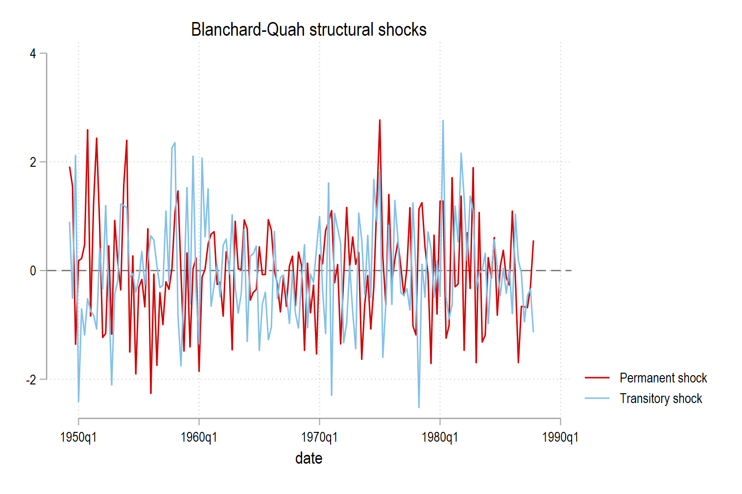

Blanchard–Quah permanent and transitory structural shocks over time — **Figure 1.** Historical realizations of the permanent and transitory shocks identified by the Blanchard–Quah long-run restriction. These are standardized structural innovations indexed by calendar time; they are not impulse responses or historical contributions.

How to read the figure

At each date, the red line reports the realization of the permanent structural shock and the blue line reports the realization of the transitory structural shock. Both series fluctuate around zero because they are innovations. Values close to +2 or −2 indicate comparatively large structural disturbances in standard-deviation units.

A value of 2 for the permanent shock does not mean that GDP growth rose by two percentage points. The contemporaneous effect on GDP growth depends on the relevant element of the impact matrix \(B\), and subsequent effects depend on the full VAR dynamics.

The figure should also not be interpreted as a historical decomposition. To obtain the contribution of each shock to GDP growth or unemployment, the innovations must be propagated through the moving-average representation of the VAR. The graph instead shows the underlying sequence of structural innovations before that dynamic propagation.

A qualification about the economic labels

The labels “permanent” and “transitory” follow directly from the long-run zero restriction. In the conventional interpretation of Blanchard and Quah (1989), they are called supply and demand shocks. However, the sign of each identified shock remains a normalization choice: multiplying one column of \(B\) and the corresponding shock series by −1 leaves the model unchanged.

For this reason, the safest labels at the extraction stage are permanent shock and transitory shock. Interpreting a positive realization as an expansionary supply or demand disturbance requires checking the corresponding impulse responses and adopting an explicit sign normalization.

What changes with sign and narrative restrictions?

The Blanchard–Quah model is point identified conditional on the VAR specification, variable ordering, and normalization, so it yields one structural-shock history. Sign and narrative restrictions are different: they generally identify a set of admissible structural models. There is therefore no unique structural-shock series unless one selects a complete accepted draw or carries all accepted draws into the subsequent analysis.

This distinction is important. A pointwise median calculated across structural-shock histories need not correspond to any single admissible structural model. For a second-stage regression or local projection, the most rigorous procedure is to repeat the analysis across accepted draws and report the resulting distribution of estimates.

Conclusion

The VAR_NR package already contains everything needed to recover the historical structural innovations. The essential step is to use the identified impact matrix and solve

\varepsilon_t=B^{-1}u_t.

In practice, the key Mata line is:

eps_bq = lusolve(VAR.inv_B0,VAR.U')'

After aligning the rows with the effective VAR sample, st_store() transfers the structural innovations back into ordinary Stata variables. We can then plot, inspect, export, and reuse them while preserving their original calendar dates.

Complete Stata code

The complete code below estimates the VAR, computes the IRFs and their bands, recovers the structural innovations, checks the date alignment, validates the reconstruction, labels the shocks, plots them, and saves them in a separate dataset.

**# /* Long-run Zero Restrictions */

clear *
use data_longrun, clear
tsset date

// -----------------------------------------------------------------------------
// Estimate the reduced-form VAR
// -----------------------------------------------------------------------------

var GDPGrowth Unemployment, lags(1/4)

// Construct the VAR_NR objects using Blanchard-Quah identification
var_nr bq, varname("VAR") optname("opts")

// Change and display options
var_nr_options, optname("opts") savefmt("png") pctg(68)
var_nr_options_display, optname("opts") all

// -----------------------------------------------------------------------------
// IRFs and confidence bands
// -----------------------------------------------------------------------------

var_nr_irf, varname("VAR") optname("opts") ///
    outname("IRF") statamatrix("IRF")

set seed 123456

var_nr_irf_bands, varname("VAR") optname("opts") ///
    outname("IRFB")

// -----------------------------------------------------------------------------
// Create variables that will receive the structural shocks
// -----------------------------------------------------------------------------

capture drop shock_bq_permanent shock_bq_transitory

generate double shock_bq_permanent = .
generate double shock_bq_transitory = .

// -----------------------------------------------------------------------------
// Plot the IRFs and recover the structural shocks
// -----------------------------------------------------------------------------

mata

// Plot only the responses associated with GDP growth
opts.shck_plt = "GDPGrowth"
irf_plot(IRF,IRFB,VAR,opts)

// Reconstruct the Blanchard-Quah contemporaneous impact matrix
VAR.inv_B0 = J(0,0,.)
identify(VAR,opts)

// Recover structural innovations: dates in rows, shocks in columns
eps_bq = lusolve(VAR.inv_B0,VAR.U')'

// Align the residual sample with the observations in the Stata dataset
first_obs_bq = VAR.nobs - rows(eps_bq) + 1
obs_bq = (first_obs_bq::VAR.nobs)

// Check the alignment before transferring the shocks
if (rows(eps_bq)!=rows(obs_bq)) {
    _error("BQ structural-shock/sample alignment failed")
}

// Transfer the structural innovations to Stata
st_store(obs_bq,("shock_bq_permanent","shock_bq_transitory"),eps_bq)

// Retain the contemporaneous impact matrix
st_matrix("B_bq",VAR.inv_B0)

// Check that B*epsilon reproduces the reduced-form innovations
reconstruction_error_bq = max(abs(vec(VAR.U' - VAR.inv_B0*eps_bq')))
st_numscalar("bq_reconstruction_error",reconstruction_error_bq)

end

// -----------------------------------------------------------------------------
// Labels and diagnostics
// -----------------------------------------------------------------------------

label variable shock_bq_permanent ///
    "BQ shock 1: permanent shock"

label variable shock_bq_transitory ///
    "BQ shock 2: transitory shock"

matrix rownames B_bq = GDPGrowth Unemployment
matrix colnames B_bq = permanent transitory

matrix list B_bq

display "Maximum BQ reconstruction error = " ///
    %12.4e scalar(bq_reconstruction_error)

summarize shock_bq_permanent shock_bq_transitory
correlate shock_bq_permanent shock_bq_transitory

// -----------------------------------------------------------------------------
// Plot and export the structural shocks
// -----------------------------------------------------------------------------

tsline shock_bq_permanent shock_bq_transitory, ///
    yline(0, lpattern(dash))                   ///
    title("Blanchard-Quah structural shocks") ///
    legend(order(1 "Permanent shock"           ///
                 2 "Transitory shock"))        ///
    name(bq_structural_shocks, replace)

graph export "bq_structural_shocks.png", ///
    replace width(3000)

// -----------------------------------------------------------------------------
// Save the structural-shock series
// -----------------------------------------------------------------------------

preserve

keep date shock_bq_permanent shock_bq_transitory
drop if missing(shock_bq_permanent)
compress

save "bq_structural_shocks.dta", replace

restore

Practical point: run the entire Mata block—from mata to end—as one block. Running only part of it from the Do-file Editor can produce an “end statement missing” error and leave intermediate Mata objects undefined.