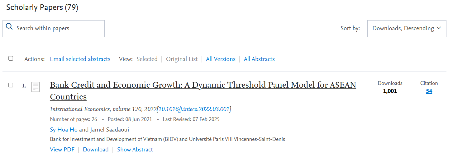
Our paper, Bank Credit and Economic Growth: A Dynamic Threshold Panel Model for ASEAN Countries, recently crossed the symbolic threshold of 1,000 SSRN downloads. The screenshot I saved at that moment showed 1,001 downloads and placed the paper first on my SSRN profile when the list was sorted by downloads. This milestone provided a good reason to reopen the replication files and ask whether the original nonlinear result survives under a newer panel-data estimator.
A second motivation came from my participation in the
31st International Panel Data Conference, held
at the University of Exeter on July 6–7, 2026. I presented another applied
macroeconomics paper in a session that also included Jan Ditzen. The conference
was a natural setting in which to revisit an older panel-threshold application
using the new community-contributed Stata command
xtthreshold.
Main result. The new estimator places the threshold at 96.2% of GDP, almost exactly the 96.5% estimate in our published paper. Below the threshold, the conditional association between bank credit and growth is positive; above it, the new pooled CCE estimate is negative.
What the original paper found
The paper, co-authored with Sy-Hoa Ho and published in International Economics in 2022, studies seven ASEAN countries over 1993–2019. We estimate a dynamic panel threshold model in which the short-run relationship between bank credit and GDP-per-capita growth can change when the credit-to-GDP ratio crosses an unknown value. The original estimator also allows a group of explanatory variables to be endogenous.
The published results place the threshold at approximately 96.5% of GDP. At or below that value, the short-run coefficient on bank credit is positive, approximately 0.08, and statistically significant. Above the threshold, it falls to approximately 0.01 and is not statistically significant in the published baseline. The central conclusion is therefore nonlinear: additional bank credit contributes much less to growth once credit is already high relative to GDP.
The article is available through its DOI, while the working-paper version remains available on SSRN.
What xtthreshold adds
The new exercise addresses a different econometric concern: unobserved common shocks that affect all countries, but with different intensities. Global financial conditions, commodity prices, regional demand, and other shared developments can generate cross-sectional dependence in a panel of ASEAN economies. An interactive-fixed-effects specification represents these common forces through latent factors with country-specific loadings.
The static threshold model with interactive fixed effects is easier to read in two steps. First, GDP-per-capita growth depends on bank credit, the observed controls, and unobserved common factors:
The coefficient on bank credit changes when the credit-to-GDP ratio crosses the unknown threshold:
Here, \(g_{it}\) is GDP-per-capita growth, \(c_{it}\) is the credit-to-GDP ratio, and \(\gamma\) is the unknown threshold. The vector \(\mathbf{x}_{it}\) contains the controls whose coefficients remain constant across regimes. The coefficients \(\beta_L\) and \(\beta_H\) measure the credit–growth relationship below and above the threshold. Finally, \(\boldsymbol{\lambda}_{i}^{\prime}\mathbf{f}_{t}\) captures unobserved common shocks through common factors with country-specific loadings.
In the threshold-search stage, the cross-sectional-average term is \(\bar c_t=N^{-1}\sum_{i=1}^{N}c_{it}\), the cross-sectional average of the credit-to-GDP ratio. In the final pooled CCE regression, the augmentation uses both \(\bar g_t\), the cross-sectional average of GDP-per-capita growth, and \(\bar c_t\). The remaining controls are not included among the CSA variables in this application.
xtthreshold combines a threshold search with the common
correlated effects, or CCE, approach. Cross-sectional averages of observed
variables proxy the unobserved common-factor space. For each candidate value of
the threshold, the command estimates the CCE-transformed model and computes its
residual sum of squares. It selects the candidate that minimizes that objective.
The theory, inference, and Monte Carlo analysis are developed by Jan Ditzen, Yiannis Karavias, and Joakim Westerlund in their open-access article, “Threshold Regression for Fixed-T Panel Data with Interactive Fixed Effects,” published in the Oxford Bulletin of Economics and Statistics.
This is a re-estimation and sensitivity exercise, not an exact replication of the published dynamic GMM model. The new specification is static: it omits the lagged dependent variable and does not reproduce the original internal-instrument strategy. The two approaches therefore answer related, but not identical, econometric questions.
Data and empirical specification
The balanced panel contains 189 observations: seven countries observed over 27 years, from 1993 to 2019. The countries are Brunei Darussalam, Indonesia, Malaysia, the Philippines, Singapore, Thailand, and Vietnam.
The dependent variable is the annual growth rate of GDP per capita. The threshold variable is the credit-to-GDP ratio. Its coefficient is allowed to change across the low-credit and high-credit regimes. The remaining controls have coefficients that are constant across regimes:
- the annual percentage change in investment;
- the annual percentage change in government expenditure;
- the terms of trade;
- the openness ratio; and
- CPI inflation.
Estimating the threshold in Stata
The required packages can be installed from Jan Ditzen’s repositories:
ssc install moremata, replace

net install xtthreshold, ///
    from("https://janditzen.github.io/xtthreshold/") replace

net install xtdcce2, ///
    from("https://janditzen.github.io/xtdcce2/") replace
The central threshold specification is:
global XTTH_Y gdpgpc
global XTTH_Z creditgdp
global XTTH_CONTROLS inv gov tot open inflation

* Threshold search: use the CSA of credit-to-GDP only.
global XTTH_CSA ${XTTH_Z}
global XTTH_GRID 90

xtthreshold ${XTTH_Y} ${XTTH_Z} | ${XTTH_CONTROLS}, ///
    threshold(${XTTH_Z}) ///
    csa(${XTTH_CSA}) ///
    grid(${XTTH_GRID})
The location of a variable relative to the vertical bar is important. The
coefficient on creditgdp, which appears before the bar, is allowed
to differ across regimes. The controls placed after the bar retain constant
coefficients. The option threshold(creditgdp) defines the variable
that separates the regimes, while csa(creditgdp) adds the
cross-sectional average of the threshold variable during the threshold search.
A threshold of 96.2% of GDP
The new estimate is 96.2% of GDP. On the 90-point search grid, this is the only candidate value inside the reported 95% likelihood-ratio confidence set. It is strikingly close to the 96.5% threshold obtained with the original dynamic-panel estimator: the difference is only about 0.3 percentage point.
The likelihood-ratio profile shows how the threshold is selected. The solid line gives the LR statistic for each candidate value of \(\gamma\). The statistic is normalized to zero at the minimizing value, 96.2. The dashed horizontal line is the 95% critical value of 7.35. Candidate thresholds below that line constitute the grid-based confidence set.
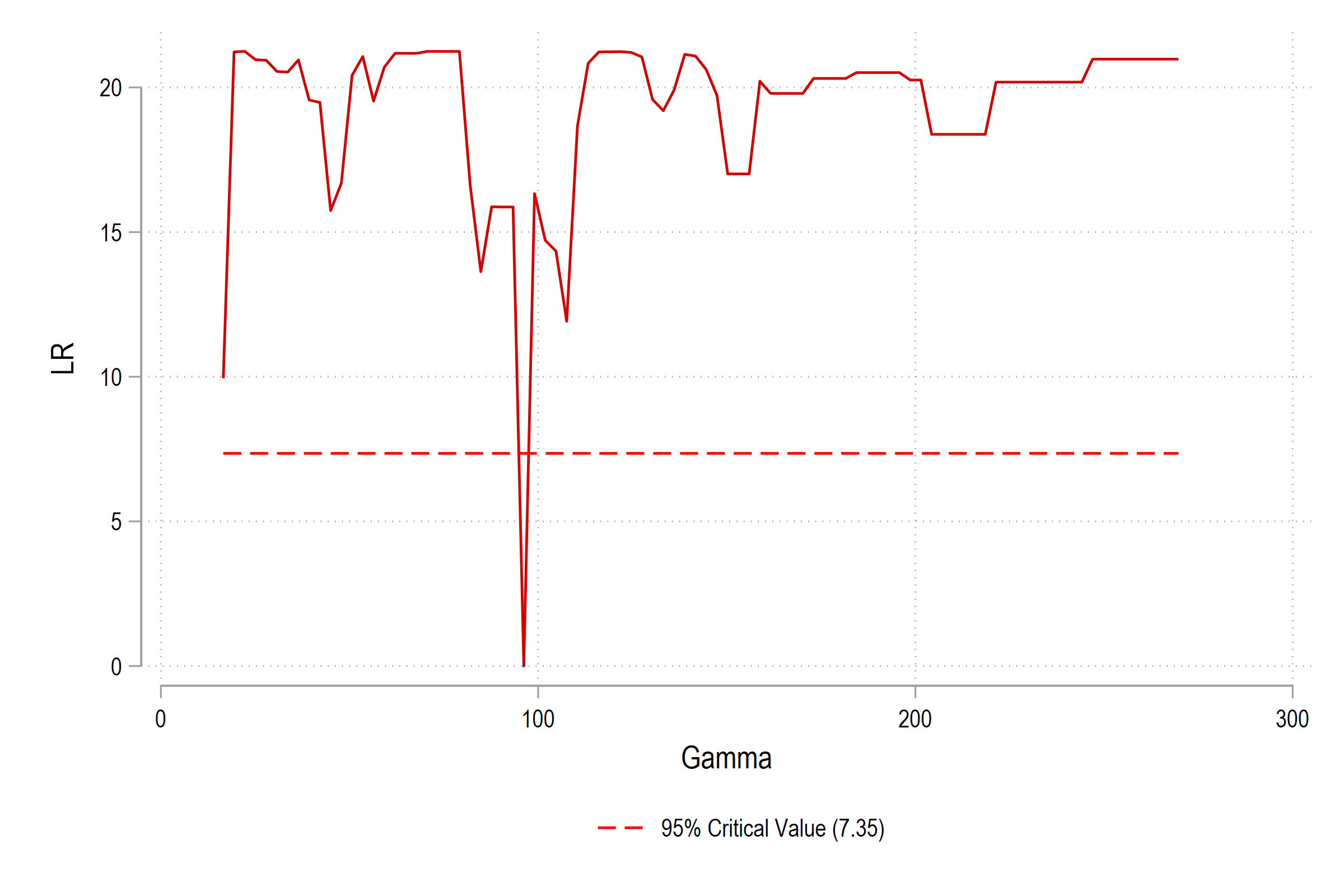
The estimated threshold divides the sample into 108 observations below the threshold, or 57.1% of the sample, and 81 observations above it, or 42.9%. Brunei Darussalam, Indonesia, and the Philippines remain below the threshold throughout the sample; Malaysia and Thailand remain above it; Singapore and Vietnam provide within-country movements between the two regimes.
Regime composition by country
| Country | Below threshold | Above threshold | Total |
|---|---|---|---|
| Brunei Darussalam | 27 | 0 | 27 |
| Indonesia | 27 | 0 | 27 |
| Malaysia | 0 | 27 | 27 |
| Philippines | 27 | 0 | 27 |
| Singapore | 10 | 17 | 27 |
| Thailand | 0 | 27 | 27 |
| Vietnam | 17 | 10 | 27 |
| Total | 108 | 81 | 189 |
Estimating the regime-specific slopes
After estimating the threshold, estat split creates one
credit-to-GDP regressor for each regime. I then estimate the structural slopes
with pooled CCE using xtdcce2:
estat graph lr
estat split

global XTTH_SPLITVARS creditgdp_0 creditgdp_1
global XTTH_MODELVARS ${XTTH_SPLITVARS} ${XTTH_CONTROLS}

* Final CCE stage: use the CSAs of gdpgpc and creditgdp only.
xtdcce2 ${XTTH_Y} ${XTTH_MODELVARS}, ///
    cr(${XTTH_Y} ${XTTH_CSA}, cr_lags(0)) ///
    pooled(${XTTH_MODELVARS}) ///
    pooledvce(wpn) ///
    mgmissing

test creditgdp_0 = creditgdp_1
lincom creditgdp_0 - creditgdp_1
Because XTTH_CSA contains only
creditgdp, the expression
cr(${XTTH_Y} ${XTTH_CSA}, cr_lags(0)) expands to
cr(gdpgpc creditgdp, cr_lags(0)). The final equation therefore
includes the contemporaneous cross-sectional averages of GDP-per-capita growth
and the credit-to-GDP ratio—and no CSA of the five controls. The structural
slopes are pooled, whereas the constant and the coefficients on the two
cross-sectional averages may remain country-specific.
The option pooledvce(wpn) requests the
Westerlund–Petrova–Norkute fixed-T standard errors. The option
mgmissing is useful because some countries remain entirely within
one regime, making one of the split credit variables country-specifically
collinear.
| Coefficient | Estimate | Standard error | 95% confidence interval | p-value |
|---|---|---|---|---|
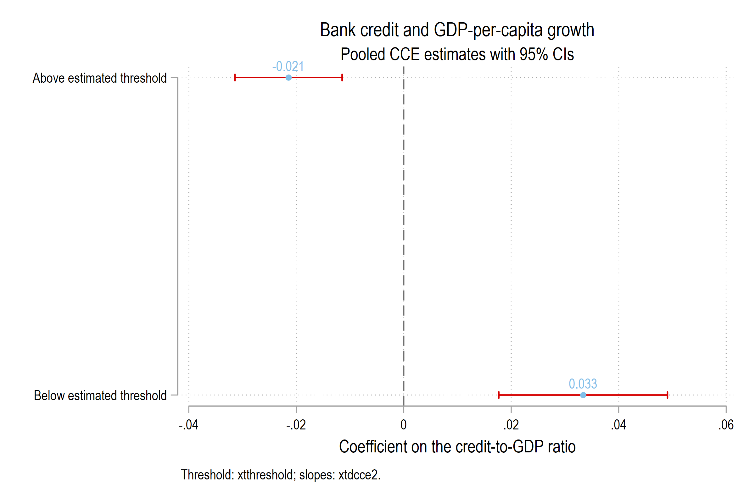
| Credit-to-GDP below 96.2% | 0.0334 | 0.0080 | [0.0177, 0.0491] | < 0.001 |
| Credit-to-GDP above 96.2% | −0.0214 | 0.0051 | [−0.0314, −0.0115] | < 0.001 |
| Difference: below minus above | 0.0548 | 0.0127 | [0.0297, 0.0800] | < 0.001 |
Economic interpretation
The new estimates indicate an estimated sign reversal in the conditional credit–growth relationship. Below the threshold, a one-percentage-point increase in the credit-to-GDP ratio is associated with a 0.033-percentage-point increase in annual GDP-per-capita growth. Above the threshold, the corresponding association is −0.021 percentage point.
A 10-percentage-point increase in credit-to-GDP is associated with about 0.33 percentage point more annual growth below the threshold, but approximately 0.21 percentage point less growth above it.
The hypothesis that the two credit coefficients are identical is strongly rejected: F(1, 161) = 18.55, with a p-value below 0.001. The estimated difference between the low-credit and high-credit slopes is 0.0548, with a 95% confidence interval from 0.0297 to 0.0800.
These coefficients should be interpreted as regime-specific conditional associations rather than as a direct causal effect. The static CCE regression does not reproduce the original dynamic GMM instrument set.
What does the cross-sectional-dependence test say?
The final model reports a CD statistic of −2.39 with a p-value of 0.017. The null of residual cross-sectional independence is therefore rejected at the 5% level, but not at the 1% level. Put differently, the evidence of remaining dependence is present at the conventional 5% threshold, but it is not robust to the stricter 1% criterion.
This result supports a measured interpretation. The cross-sectional averages of the dependent variable and the threshold variable absorb an important part of the common variation in the panel, but the test does not establish that all remaining cross-sectional dependence has disappeared.
How do the new results compare with the 2022 paper?
| Feature | Ho and Saadaoui (2022) | New xtthreshold exercise |
|---|---|---|
| Model | Dynamic panel threshold GMM | Static threshold model with interactive fixed effects |
| Estimated threshold | 96.5% of GDP | 96.2% of GDP |
| Credit slope below threshold | Positive and significant, approximately 0.08 | Positive and significant, 0.033 |
| Credit slope above threshold | Small and insignificant, approximately 0.01 | Negative and significant, −0.021 |
| Common shocks | Not modeled through interactive fixed effects | Approximated through CCE cross-sectional averages |
| Dynamic endogeneity treatment | Internal instruments in a dynamic threshold framework | Not reproduced in this static re-estimation |
The most stable finding is the location of the threshold. Two substantially different estimators place it at almost exactly the same credit-to-GDP ratio. This is the central result of the re-estimation.
The main difference concerns the high-credit regime. The published dynamic model finds that the positive growth contribution becomes small and statistically insignificant. The static interactive-effects re-estimation produces a negative and significant conditional association. This difference should not be attributed mechanically to one econometric feature. The new model changes the dynamics, the treatment of endogeneity, and the handling of common shocks simultaneously.
Policy interpretation: a threshold is not a mechanical ceiling
The 96% estimate should not be read as a universal prudential ceiling or a mechanical policy target. A threshold regression identifies a change in a conditional relationship within a particular sample and specification. The economic consequences of credit depend on its allocation, the characteristics of borrowers, banking supervision, and the productive structure of the economy.
For ASEAN economies, the composition of lending is especially important. Credit financing productive investment and export-oriented firms may have a very different growth effect from credit directed toward already leveraged households, real estate, or low-productivity activities. The result therefore reinforces the distinction between the quantity of finance and the quality and allocation of finance.
Scope and qualifications
First, the fixed-T theory is developed for panels in which the number of cross-sectional units becomes large. The present application contains only seven countries and 27 annual observations per country. It is therefore most useful as an empirical illustration and robustness exercise. Formal inference should be read with that sample structure in mind.
Second, the new regression is static and does not reproduce the dynamic instrument strategy of the original paper. The published GMM results and the new interactive-effects results should be viewed as complementary evidence, not as alternative estimates of exactly the same parameter.
Conclusion
Revisiting our ASEAN data with xtthreshold produces a strikingly
stable threshold estimate. The new value, 96.2% of GDP, is almost identical to
the 96.5% estimate reported in our 2022 paper. Below that threshold, bank credit
is positively associated with GDP-per-capita growth. Above it, the pooled CCE
estimate becomes negative.
The stability of the breakpoint across very different estimators strengthens the case for taking nonlinearities in the finance–growth relationship seriously. At the same time, the change in the high-credit coefficient shows why dynamics, endogeneity, and common shocks matter. The new Stata package makes these comparisons transparent and easy to reproduce.
Replication
The complete Stata do-file is available in the
xtthreshold_asean_blog.do
on the EconMacroBlog GitHub repository. It is designed to run from the root
of the unzipped replication package. After setting that folder as Stata’s
current working directory, run:
do xtthreshold_asean_blog.doReferences and resources
- Ho, S.-H., and J. Saadaoui (2022), “Bank Credit and Economic Growth: A Dynamic Threshold Panel Model for ASEAN Countries,” International Economics, 170, 115–128.
- Ditzen, J., Y. Karavias, and J. Westerlund (2026), “Threshold Regression for Fixed-T Panel Data with Interactive Fixed Effects,” Oxford Bulletin of Economics and Statistics.
-
xtthresholddocumentation and installation instructions. -
xtdcce2documentation. - 31st International Panel Data Conference, University of Exeter, July 6–7, 2026.
- IPDC 2026 conference program.