xtswitchdid with Stata

On 29 July 2026, Stata announced a new StataNow update introducing xtswitchdid, a built-in command for difference in differences with switching treatments. The official Stata Blog announcement highlights that the command handles binary or multivalued treatments, allows subjects to switch in and out of treatment or between treatment levels, and provides event-study effects, placebo tests, treatment-path analysis, and an average total effect. This is an important addition to Stata’s difference-in-differences toolkit because many policy treatments are neither binary nor absorbing. A country may enter an agreement, deepen it later, experience another expansion, or move back toward its initial treatment level. A state may tighten a regulation and subsequently relax it. A firm may receive several treatment doses at different dates. Standard staggered-adoption estimators are not designed for all these paths.

xtswitchdid implements the heterogeneous difference-in-differences framework developed by Clément de Chaisemartin and Xavier D’Haultfœuille for multivalued and switching treatments with potentially dynamic effects. The command estimates event-study effects by comparing the treatment path that a group actually experiences after its first change with a counterfactual path in which its treatment remains fixed at the initial level.

Main takeaway. Use xtswitchdid when the treatment can take more than two values, can change several times, or can switch out as well as in. The estimand is built around treatment paths, not merely a binary treated-versus-untreated indicator.

1. Why do we need another DID command?

Commands such as xthdidregress are particularly well suited to binary and absorbing treatments: once a group enters treatment, it remains treated. This framework covers many staggered-adoption applications, but it does not describe all policy designs.

Suppose that the treatment of group g follows one of these paths:

0 0 2 2 3 3
0 0 4 0 0 1
0 0 1 1 0 0

The first group receives a higher treatment dose and later a further increase. The second receives a large one-period change and then another smaller change. The third enters treatment and later exits. Reducing these paths to a single absorbing indicator discards economically relevant variation.

The underlying econometric motivation is also important. In complex treatment designs, conventional two-way fixed-effects event studies, distributed-lag regressions, and naive panel local projections may combine effects from different exposure lengths, assign negative weights, or use future switchers as controls after they have changed treatment. The de Chaisemartin–D’Haultfœuille estimator instead constructs transparent comparisons between switchers and groups that still maintain the same initial treatment level.

2. The actual-versus-status-quo estimand

Let \(D_{g,t}\) denote the treatment of group \(g\) in period \(t\). Define the first treatment change as

\[ F_g = \min\{t\geq 2 : D_{g,t}\neq D_{g,t-1}\}. \]

At exposure \(\ell\), the outcome is observed in period \(F_g-1+\ell\). The group-specific actual-versus-status-quo effect is

\[ \delta_{g,\ell} = \mathbb{E}\!\left[ Y_{g,F_g-1+\ell}(D_{g,1},\ldots,D_{g,F_g-1+\ell}) – Y_{g,F_g-1+\ell}(D_{g,1},\ldots,D_{g,1}) \mid \mathcal D \right]. \]

The first potential outcome follows the group’s actual treatment path. The second holds treatment permanently at its initial value. Therefore, xtswitchdid answers a direct policy question:

How did the observed sequence of treatment changes affect the outcome relative to a counterfactual in which no treatment change occurred?

For switchers-in, the command aggregates these group-level effects into

\[ \delta_{\ell} = \frac{1}{N_{\ell}} \sum_{g:F_g-1+\ell\leq T_g} \delta_{g,\ell}. \]

Exposure 1 is the first switching period, exposure 2 is one period after the first switch, exposure 3 is two periods afterward, and so forth. This timing convention differs from conventional event-study graphs in which the treatment year is often called event time 0.

3. Raw and normalized effects

By default, xtswitchdid reports normalized effects. The treatment dose accumulated by group \(g\) through exposure \(\ell\) is

\[ \Delta^D_{g,\ell} = \sum_{k=0}^{\ell-1} \left(D_{g,F_g+k}-D_{g,1}\right). \]

The normalized estimand divides the raw actual-versus-status-quo effect by the relevant average treatment dose:

\[ \delta^n_{\ell} = \frac{\delta_{\ell}}{\overline{\Delta^D}_{\ell}}. \]

Normalized effects can be interpreted as weighted averages of the effects of the current treatment and its lags per unit of treatment dose. They are useful when one wants a per-unit interpretation and the numerical treatment scale is economically meaningful.

The option raw disables this normalization. Raw effects instead measure the outcome consequence of the actual treatment packages experienced by switchers. In the empirical illustration below, I use raw because the treatment changes represent large integration packages rather than homogeneous one-unit interventions.

4. Empirical illustration: Economic Integration Agreements and growth

I illustrate the command with a country-year panel. The data and empirical setting come from the NBER working paper by Joshua Aizenman, Hiro Ito, and Jamel Saadaoui, Comparative Advantage and Openness under Global Fragmentation: Lessons from the Past 65 Years (NBER Working Paper No. 35242). The outcome is annual real GDP growth. The treatment is the annual change in the number of bilateral Economic Integration Agreement links, constructed from Mario Larch’s Regional Trade Agreements Database. The institutional-quality indicator INST is included as a covariate.

The underlying database is bilateral. Consequently, the country-year treatment counts partner relationships covered by EIAs. A jump of 17 does not necessarily mean that a country signed 17 separate legal treaties in one year. It can reflect one plurilateral or regional integration event that simultaneously activates 17 bilateral links.

I first declare the panel and construct the annual treatment change:

xtset imfcode period

generate double deia = D.eia

I use a fixed, predetermined population criterion based on population in 1990. This avoids a time-varying sample rule that could redefine a country’s observed baseline or first treatment switch.

bysort imfcode: egen double pop_base = ///
    max(cond(period == 1990, pop, .))

generate byte sample = ///
    !missing(pop_base) & pop_base >= 2

The estimation window begins in 1990. Although I use tsfill, full in the complete do-file for treatment-path diagnostics, xtswitchdid itself can work with an unbalanced panel. Adding empty rows does not create observed outcome, treatment, or covariate data.

5. The basic xtswitchdid specification

xtswitchdid (growth INST) (deia) ///
    if sample & period > 1989, ///
    group(imfcode) ///
    switchgroup(in) ///
    controlgroup(all) ///
    raw ///
    neffects(4) ///
    vce(cluster imfcode)

The syntax is compact, but each element matters:

• (growth INST) specifies the outcome followed by the covariate.
• (deia) specifies the treatment.
• group(imfcode) identifies the country as the treatment group.
• switchgroup(in) retains groups whose first treatment change is above their initial treatment level.
• controlgroup(all) uses both never-switchers and not-yet-switchers that still maintain the same baseline treatment.
• raw reports the effect of the actual treatment path rather than the effect normalized by treatment dose.
• neffects(4) estimates the treatment year and the following three periods.
• vce(cluster imfcode) clusters inference at the country level, where treatment varies.

The panel identifier and time variable are inherited from xtset. Unlike a conventional staggered DID command, there is no need to create a cohort variable: xtswitchdid identifies the first switch directly from the treatment path.

6. Why institutional quality is a useful control

Institutional development can influence both growth and a country’s capacity or willingness to enter, deepen, and implement international economic agreements. Omitting institutional changes could therefore attribute to EIA expansion a growth acceleration associated with a wider domestic reform episode.

With covariates, the identifying condition becomes conditional parallel trends. In simplified notation, the command assumes that the counterfactual growth change net of institutional changes evolves similarly for switchers and eligible controls:

\[ \mathbb{E}\!\left[ \Delta Y^0_{g,t} – \Delta INST_{g,t}\,\theta \mid \text{switcher information} \right] = \mathbb{E}\!\left[ \Delta Y^0_{c,t} – \Delta INST_{c,t}\,\theta \mid \text{control information} \right]. \]

This is not the same as adding the level of INST to an ordinary static regression. Internally, the adjustment is based on changes in the outcome and changes in the covariate among observations whose treatment has not yet changed. Switchers and controls may have different counterfactual growth trends to the extent that these differences are explained by changes in institutional quality.

7. Main dynamic results

The all-controls specification uses 3,203 observations and 101 countries after accounting for missing outcome, treatment, and institutional data. The raw effects are:

Exposure	Timing	Effect	Standard error	p-value
1	First EIA change	0.0082	0.0075	0.279
2	One year later	0.0286	0.0073	<0.001
3	Two years later	0.0130	0.0064	0.044
4	Three years later	0.0128	0.0101	0.204

Because growth is expressed in decimal units, the estimates correspond to percentage-point changes after multiplication by 100. There is no precisely estimated contemporaneous effect. The response peaks one year after the first EIA expansion at approximately 2.9 percentage points. It remains positive two years later and is still positive, though imprecisely estimated, after three years.

The dynamic effects can be plotted immediately after estimation:

estat eventplot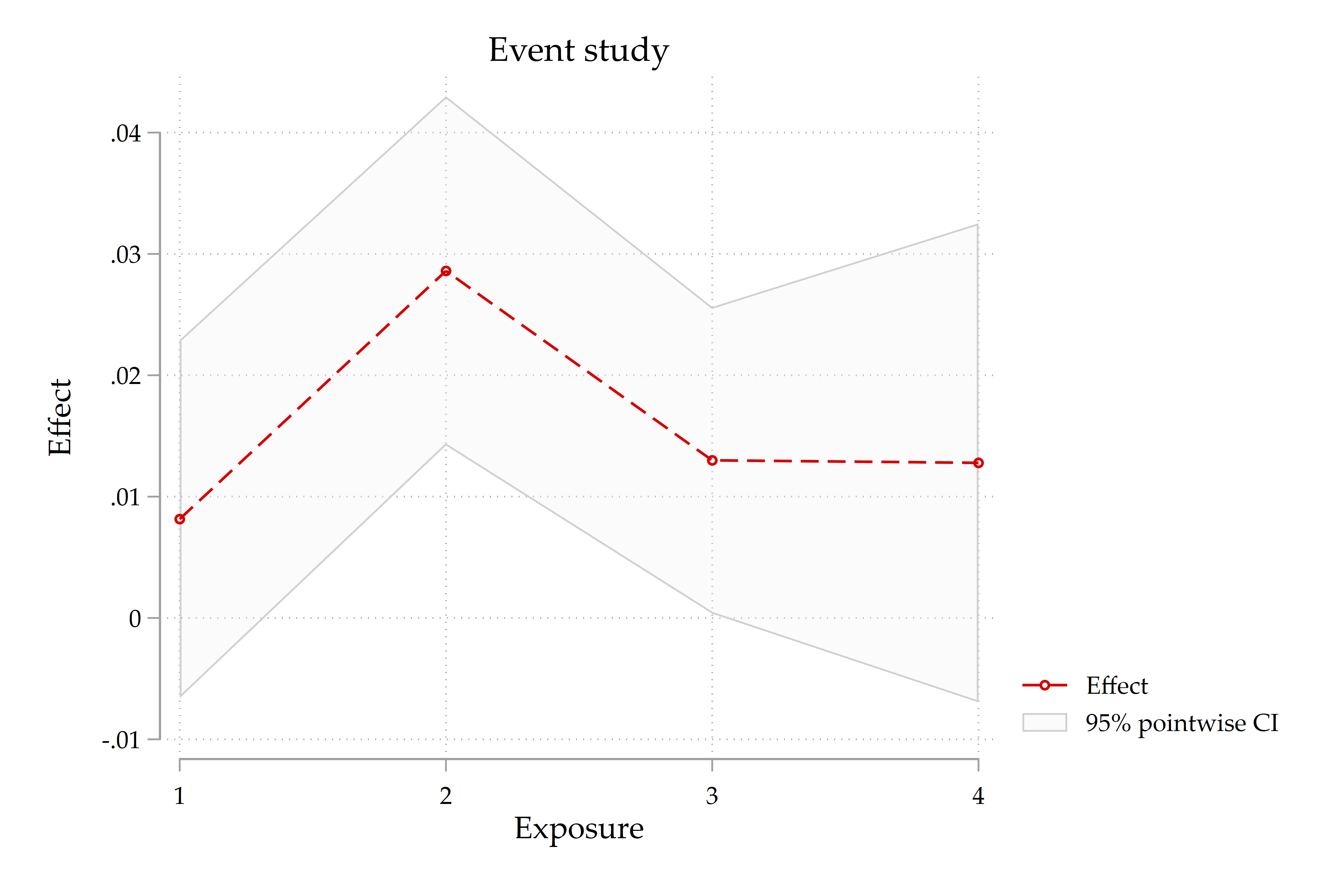

8. Placebo effects and the identifying assumptions

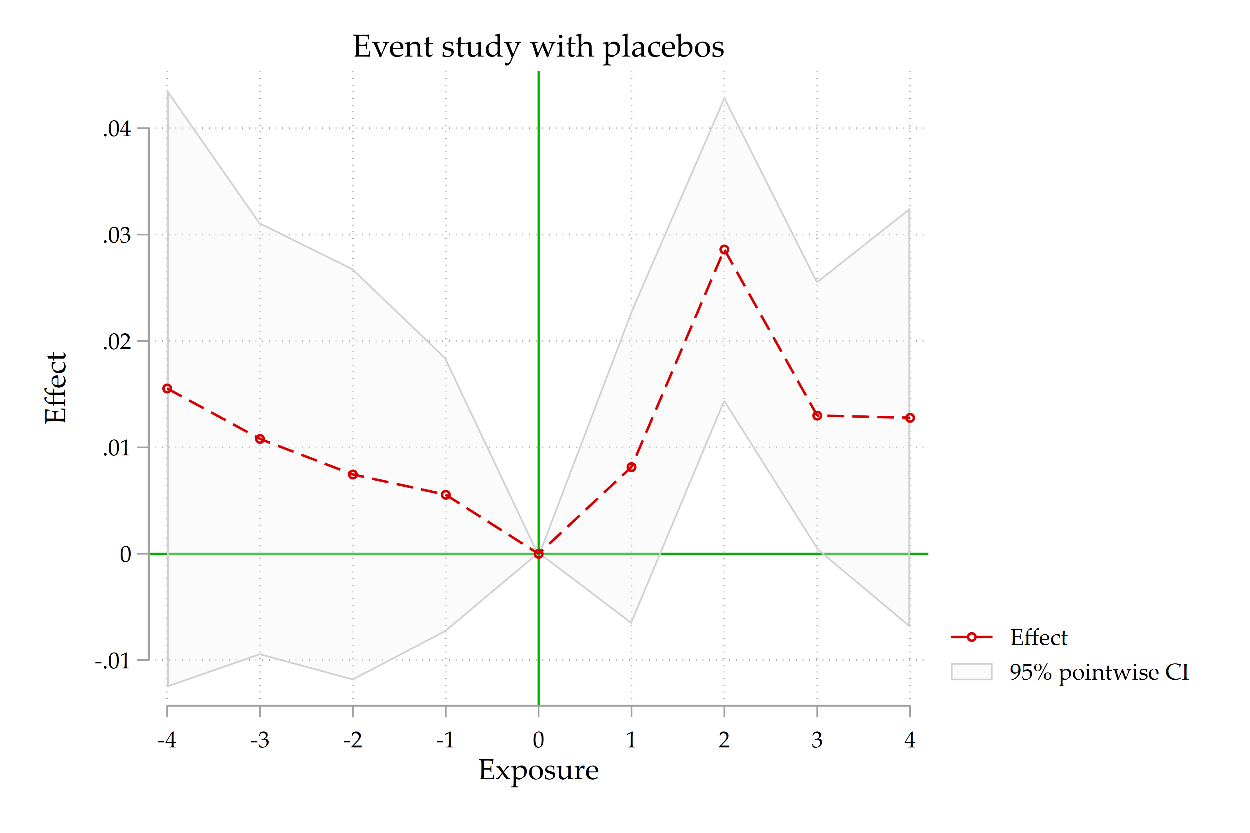
As with other DID estimators, causal interpretation relies on parallel trends and no anticipation. xtswitchdid constructs placebo effects that mimic the corresponding treatment effects over pretreatment windows.

estat ptrends

quietly estat ptrends, graph alleffects

In the all-controls specification, none of the four placebo estimates is individually significant. The joint test is

\[ \chi^2(4)=1.52, \qquad p=0.8236. \]

Thus, the data provide no evidence against conditional parallel trends and no anticipation over the four-period window. These placebo coefficients are not ordinary one-year leads. Placebo \(-\ell\) mirrors the corresponding \(\ell\)-period post-switch comparison, using a pretreatment evolution of the same length.

9. Never-switchers and a common set of switchers

The control group can be restricted to countries whose treatment never changes:

xtswitchdid (growth INST) (deia) ///
    if sample & period > 1989, ///
    group(imfcode) ///
    switchgroup(in) ///
    controlgroup(never) ///
    raw ///
    neffects(4) ///
    vce(cluster imfcode)

The option commonswitchers then holds the set of switching countries fixed across the four exposures:

xtswitchdid (growth INST) (deia) ///
    if sample & period > 1989, ///
    group(imfcode) ///
    switchgroup(in) ///
    controlgroup(never) ///
    raw ///
    neffects(4) ///
    commonswitchers ///
    vce(cluster imfcode)

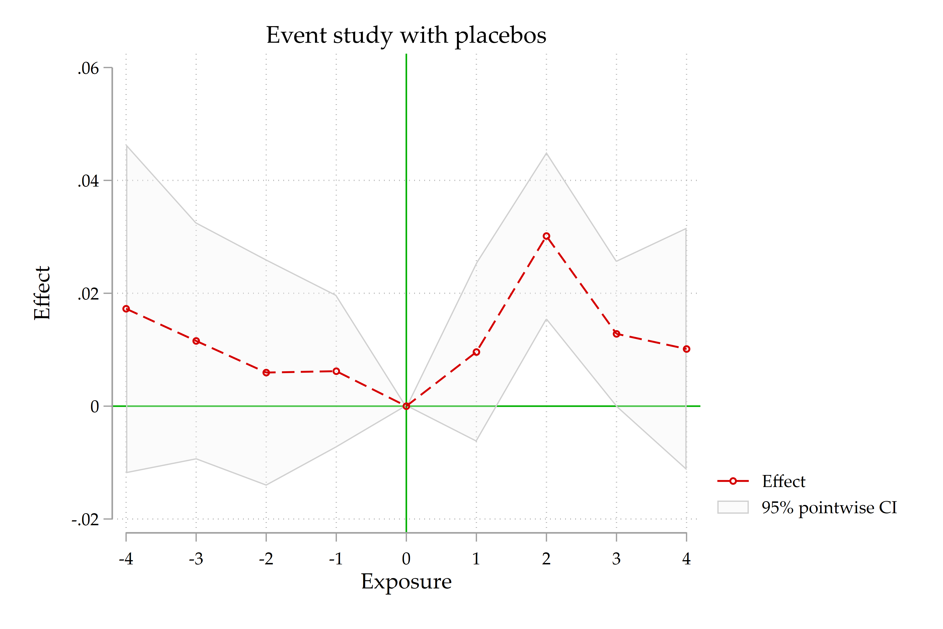
The estimates are very stable:

Specification	Exposure 1	Exposure 2	Exposure 3	Exposure 4	Joint placebo p
All eligible controls	0.0082	0.0286	0.0130	0.0128	0.824
Never-switcher controls	0.0100	0.0301	0.0128	0.0101	0.779
Never controls, common switchers	0.0096	0.0301	0.0128	0.0101	0.774

The common-switcher specification contains 28 switching countries. The near equality of the second and third rows shows that the event-study profile is not generated by a changing composition of switchers across horizons.

10. The average total effect

estat total aggregates the dynamic effects into an average total effect per unit of treatment:

estat total

The population parameter can be written schematically as

\[ \delta = \frac{ \displaystyle \sum_g\sum_{\ell}\delta_{g,\ell} }{ \displaystyle \sum_g\sum_{\ell} \left(D_{g,F_g-1+\ell}-D_{g,1}\right) }. \]

The estimate is 0.00346 with all eligible controls, 0.00350 with never-switcher controls, and 0.00353 with never-switcher controls and common switchers. The corresponding p-values range from 0.010 to 0.013.

In percentage-point terms, the estimate is approximately 0.35 percentage point per incremental EIA link, accumulated over the post-switch periods entering the calculation. It is not an annual effect of 0.35 percentage point in every subsequent year.

11. Treatment paths are part of the result

One of the most useful postestimation commands is

estat paths, pathlen(4)

For the 28 common switchers, the treatment paths are:

Treatment path	Countries	Share
0 17 0 0 0	15	53.6%
0 27 0 0 3	4	14.3%
0 30 0 0 0	2	7.1%
0 8 1 0 0	7	25.0%

This table is essential for interpretation. The raw coefficient is not the marginal effect of signing one additional bilateral treaty. It averages the effects of the observed integration paths relative to no change in EIA exposure.

The concentration in large regional paths is not necessarily a problem. The history of globalization is organized around large institutional blocs rather than a sequence of equal and independent bilateral agreements. This is consistent with the idea of hegemonic globalization developed by Broner, Martín, Meyer, and Trebesch: large powers and institutional centers promote policy alignment and deeper trade integration. The EIA event study should therefore be interpreted as evidence on major bloc-based integration episodes rather than as a universal treatment effect for every possible trade agreement.

The individual-agreement version of Mario Larch’s database can be used to map each path to the precise legal event, entry date, enlargement, or reclassification that generated the country-level jump.

Why Korea produces a short path

South Korea displays a treatment change of +10 followed by −10. Because deia is a first difference, this path moves above and then below its initial value. After a path has crossed both sides of the baseline, the actual-versus-status-quo effect can become a sign-reversing combination of positive and negative treatment increments. xtswitchdid therefore stops using that group at later exposures. Korea contributes to exposure 1 but is removed by commonswitchers, which explains the path 0 10 . . . in the unrestricted path table.

12. Leave-one-switcher-out robustness

A useful influence diagnostic is to remove each common switching country in turn and reestimate the preferred Exposure 2 effect. The benchmark estimate is 0.03015. Across all 28 leave-one-switcher-out estimations:

• all 28 estimations succeed;
• the coefficient ranges from 0.02699 to 0.03280;
• the largest absolute change is 10.49%;
• all 28 coefficients remain positive;
• all 28 remain statistically significant at the 5% level.

The largest downward change occurs when Thailand is removed, but the estimate remains 0.02699 with a p-value of 0.0001. The result is therefore not driven by any single switching country.

When automating this exercise, estimates should be extracted from e(b) and e(V), which remain available after a quiet estimation:

matrix B_LOO = e(b)
matrix V_LOO = e(V)

local b2  = el(B_LOO, 1, 2)
local se2 = sqrt(el(V_LOO, 2, 2))
local p2  = 2 * normal(-abs(`b2' / `se2'))

13. Excluding Sub-Saharan African controls

A further robustness check removes Sub-Saharan African countries from the sample of eligible controls:

xtswitchdid (growth INST) (deia) ///
    if sample & period > 1989 & ssa != 1, ///
    group(imfcode) ///
    switchgroup(in) ///
    controlgroup(all) ///
    raw ///
    neffects(4) ///
    vce(cluster imfcode)

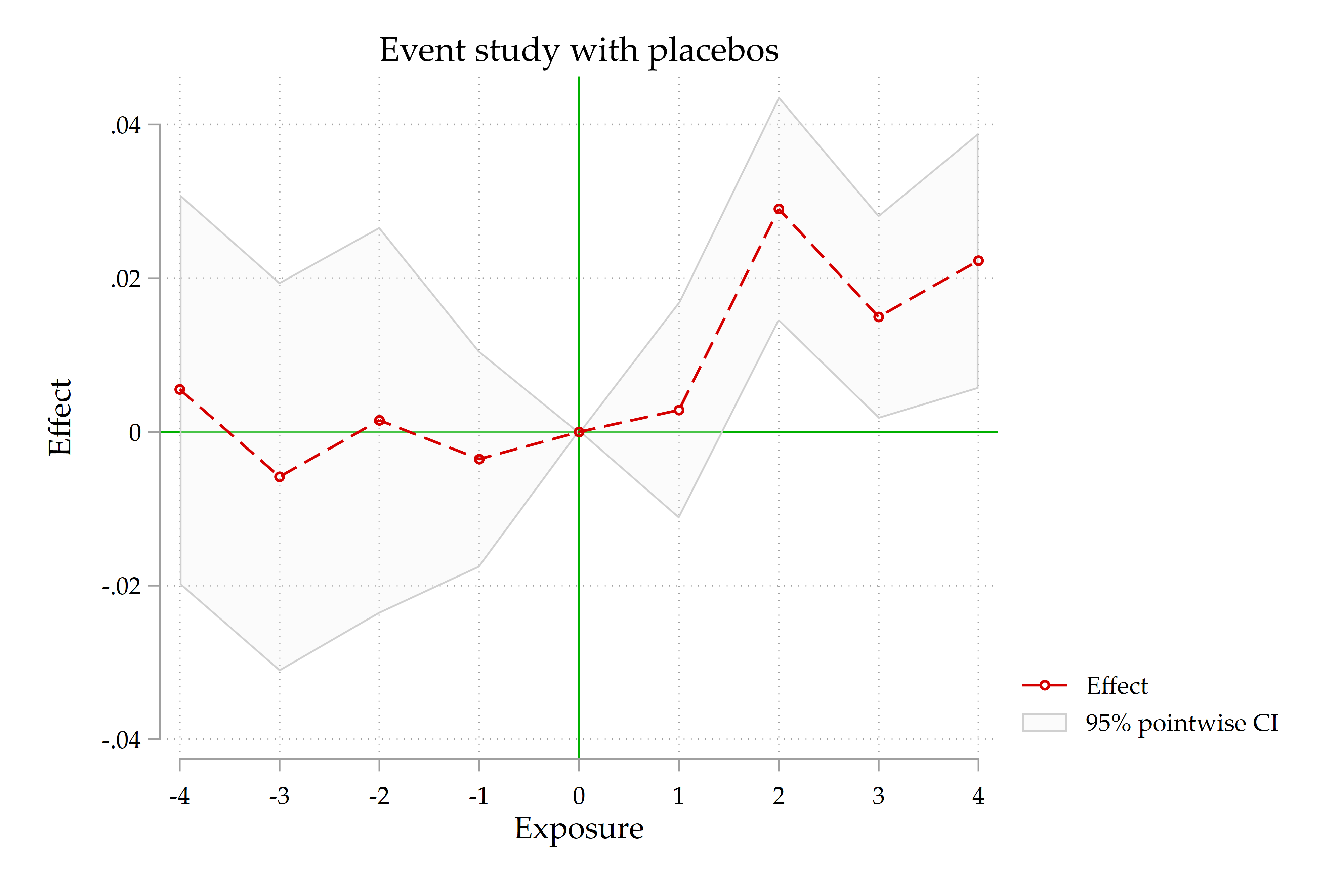
The one-year effect remains approximately 2.9 percentage points. The two- and three-year effects are also positive and statistically significant. The joint placebo test has a p-value of 0.603, and the average total effect rises modestly to 0.00381 with a p-value of 0.004.

14. A practical workflow

A transparent xtswitchdid application should follow a simple sequence:

1. Declare the panel using xtset.
2. Inspect the treatment variable and determine whether it is binary, multivalued, absorbing, or switching.
3. Define a fixed estimation sample that does not alter treatment timing.
4. Choose switchgroup(in), switchgroup(out), or both according to the research question.
5. Decide whether the substantive estimand is the raw treatment-path effect or the normalized per-dose effect.
6. Inspect estat paths rather than treating the treatment variable as a black box.
7. Report estat ptrends and explain that the placebos mirror the post-treatment horizons.
8. Compare controlgroup(all) with controlgroup(never).
9. Use commonswitchers when comparing the dynamic profile across exposures.
10. Check whether one switching group drives the main result.

15. Conclusion

xtswitchdid fills an important gap in Stata’s causal-inference toolkit. It provides a built-in event-study estimator for panel treatments that may be multivalued, nonabsorbing, and dynamically consequential. Its main advantage is not merely computational. It forces the researcher to think explicitly about the observed treatment paths and the counterfactual status-quo path.

In the EIA illustration, growth does not respond significantly in the switching year but rises strongly one year later. The result is stable across control groups, common-switcher restrictions, the exclusion of Sub-Saharan African controls, and 28 leave-one-switcher-out estimations. The placebo tests are clean over the four-period window. The economically correct interpretation is a delayed growth response to large, bloc-based expansions in formal economic integration.

References

Aizenman, J., Ito, H., and Saadaoui, J. (2026). “Comparative Advantage and Openness under Global Fragmentation: Lessons from the Past 65 Years.” NBER Working Paper No. 35242. NBER page.

Broner, F., Martín, A., Meyer, J., and Trebesch, C. (2025). “Hegemonic Globalization.” CEPR Discussion Paper 20339. CEPR page.

de Chaisemartin, C., and D’Haultfœuille, X. (2026). “Difference-in-Differences Estimators of Intertemporal Treatment Effects.” Review of Economics and Statistics, 108, 863–880. DOI.

Egger, P. H., and Larch, M. (2008). “Interdependent Preferential Trade Agreement Memberships: An Empirical Analysis.” Journal of International Economics, 76(2), 384–399. Mario Larch’s Regional Trade Agreements Database.

MacDonald, K. (2026). “A new update to StataNow has just been released.” The Stata Blog, 29 July 2026. StataNow update announcement.

StataCorp. “xtswitchdid — Difference in differences with switching treatments for panel data.” StataNow reference manual.

. 
. clear

. 
. use DATA\DATA_Apr26.dta, clear

. 
. // The panel and time variables must be declared with xtset
. xtset imfcode period

Panel variable: imfcode (unbalanced)
 Time variable: period, 1960 to 2024, but with gaps
         Delta: 1 unit

. 
. xtdes

 imfcode:  111, 112, ..., 968                                n =        200
  period:  1960, 1961, ..., 2024                             T =         65
           Delta(period) = 1 unit
           Span(period)  = 65 periods
           (imfcode*period uniquely identifies each observation)

Distribution of T_i:   min      5%     25%       50%       75%     95%     max
                         6      24      54        61        65      65      65

     Freq.  Percent    Cum. |  Pattern
 ---------------------------+-------------------------------------------------------------------
       84     42.00   42.00 |  11111111111111111111111111111111111111111111111111111111111111111
       28     14.00   56.00 |  ..........1111111111111111111111111111111111111111111111111111111
        6      3.00   59.00 |  ......11111111111111111111111111111111111111111111111111111111111
        5      2.50   61.50 |  ...................................111111111111111111111111111111
        3      1.50   63.00 |  .........................................111111111111111111111111
        3      1.50   64.50 |  .......1111111111111111111111111111111111111111111111111111111111
        3      1.50   66.00 |  .....111111111111111111111111111111111111111111111111111111111111
        3      1.50   67.50 |  ....1111111111111111111111111111111111111111111111111111111111111
        2      1.00   68.50 |  .....................................1111111111111111111111111111
       63     31.50  100.00 | (other patterns)
 ---------------------------+-------------------------------------------------------------------
      200    100.00         |  XXXXXXXXXXXXXXXXXXXXXXXXXXXXXXXXXXXXXXXXXXXXXXXXXXXXXXXXXXXXXXXXX

. 
. // -----------------------------------------------------------------------------
. // Main specification: change in EIA signature as a treatment
. // -----------------------------------------------------------------------------
. 
. gen deia = d.eia
(432 missing values generated)

. 
. // Balance the panel
. 
. tsfill, full

. 
. tsset imfcode period

Panel variable: imfcode (strongly balanced)
 Time variable: period, 1960 to 2024
         Delta: 1 unit

. 
. xtline deia, overlay legend(off) name(eia, replace)

. 
. ********************************************************************************
. 
. bysort imfcode: egen double pop_base = ///
>     max(cond(period == 1990, pop, .))
(2,405 missing values generated)

. 
. generate byte sample = ///
>     !missing(pop_base) & pop_base >= 2

. 
. assert sample == 0 if missing(pop_base)

. 
. egen byte tag_country = tag(imfcode)

. 
. count if tag_country & missing(pop_base)
  37

. count if tag_country & sample
  112

. 
. drop tag_country        

. 
. bysort imfcode: egen double eia_1989 = ///
>     max(cond(period == 1989, eia, .))
(2,470 missing values generated)

. 
. egen byte tag_country = tag(imfcode)

. 
. tabulate eia_1989 if tag_country & sample, missing

   eia_1989 |      Freq.     Percent        Cum.
------------+-----------------------------------
          0 |        111       99.11       99.11
          . |          1        0.89      100.00
------------+-----------------------------------
      Total |        112      100.00

. 
. drop tag_country

. 
. generate byte complete_case = ///
>     sample & period >= 1990 & ///
>     !missing(growth, INST, deia)

. 
. bysort imfcode: egen first_complete_year = ///
>     min(cond(complete_case, period, .))
(6,435 missing values generated)

. 
. egen byte tag_country = tag(imfcode)

. 
. tabulate first_complete_year if tag_country & sample, missing

first_compl |
   ete_year |      Freq.     Percent        Cum.
------------+-----------------------------------
       1990 |         94       83.93       83.93
       1991 |          1        0.89       84.82
       1993 |          2        1.79       86.61
       1995 |          1        0.89       87.50
       1998 |          3        2.68       90.18
          . |         11        9.82      100.00
------------+-----------------------------------
      Total |        112      100.00

. 
. drop tag_country

. 
. bysort imfcode: egen double min_deia = ///
>     min(cond(sample & period >= 1990, deia, .))
(5,720 missing values generated)

. 
. bysort imfcode: egen double max_deia = ///
>     max(cond(sample & period >= 1990, deia, .))
(5,720 missing values generated)

. 
. generate byte crosses_zero = ///
>     min_deia < 0 & max_deia > 0 ///
>     if sample
(5,720 missing values generated)

. 
. egen byte tag_country = tag(imfcode)

. 
. tabulate crosses_zero if tag_country & sample, missing

crosses_zer |
          o |      Freq.     Percent        Cum.
------------+-----------------------------------
          0 |         81       72.32       72.32
          1 |         31       27.68      100.00
------------+-----------------------------------
      Total |        112      100.00

. 
. drop tag_country

. 
. bysort imfcode: egen first_deia_switch = ///
>     min(cond(sample & period >= 1991 & ///
>     deia != 0 & !missing(deia), period, .))
(10,985 missing values generated)

. 
. generate byte switch_before_complete = ///
>     first_deia_switch < first_complete_year ///
>     if !missing(first_deia_switch, first_complete_year)
(11,115 missing values generated)

. 
. egen byte tag_country = tag(imfcode)

. 
. tabulate switch_before_complete ///
>     if tag_country & sample, missing

switch_befo |
re_complete |      Freq.     Percent        Cum.
------------+-----------------------------------
          0 |         29       25.89       25.89
          . |         83       74.11      100.00
------------+-----------------------------------
      Total |        112      100.00

. 
. drop tag_country

. 
. ********************************************************************************
.         
. xtswitchdid (growth INST) (deia) if sample & period>1989, ///
>     group(imfcode) ///
>     switchgroup(in) ///
>     controlgroup(all) ///
>         raw ///
>         neffects(4) ///
>     vce(cluster imfcode)

Treatment and time information

Panel variable:  imfcode
Time variable:   period
Time interval:   1990 thru 2024

Treatment level: imfcode
Control:         deia maintaining baseline
Treatment:       deia changing from baseline
Switchers:       switchers-in only

-----------------------------------------------------------------
Initial      |
treatment    |      Groups          Obs    Switch in    Absorbing
-------------+---------------------------------------------------
           0 |         101        3,203   1 3 8 9 ..           No
-----------------------------------------------------------------

DID with switching treatments                         Number of obs    = 3,203
                                                      Number of panels =   101
                                                      Number of groups =   101

                              (Std. err. adjusted for 101 clusters in imfcode)
------------------------------------------------------------------------------
             |               Robust
             |     Effect   std. err.      z    P>|z|     [95% conf. interval]
-------------+----------------------------------------------------------------
    Exposure |
          1  |   .0081544   .0075312     1.08   0.279    -.0066065    .0229152
          2  |   .0286051   .0073439     3.90   0.000     .0142113     .042999
          3  |   .0129914    .006449     2.01   0.044     .0003515    .0256312
          4  |   .0127839   .0100717     1.27   0.204    -.0069564    .0325242
------------------------------------------------------------------------------
Note: Effects computed using covariates.

. 
. estimates store XTS_DEIA_ALL

. 
. // Dynamic effects only
. estat eventplot

. graph export FIGURES\Figure_XTSWITCHDID_XTS_DEIA_ALL.png, ///
>     as(png) replace width(4000)
file FIGURES\Figure_XTSWITCHDID_XTS_DEIA_ALL.png saved as PNG format

. 
. // Placebo estimates and joint pretrend/no-anticipation test
. estat ptrends

Placebo estimates                                     Number of obs    = 3,203
                                                      Number of panels =   101
                                                      Number of groups =   101

                              (Std. err. adjusted for 101 clusters in imfcode)
------------------------------------------------------------------------------
             |               Robust
     Placebo |     Effect   std. err.      z    P>|z|     [95% conf. interval]
-------------+----------------------------------------------------------------
          -4 |   .0155433   .0143358     1.08   0.278    -.0125545     .043641
          -3 |   .0107999   .0103688     1.04   0.298    -.0095226    .0311223
          -2 |    .007455   .0098731     0.76   0.450    -.0118959    .0268059
          -1 |   .0055524   .0065714     0.84   0.398    -.0073274    .0184322
------------------------------------------------------------------------------

Test of parallel-trends and no-anticipation assumptions
H0: Placebos are zero for all exposures

    chi2(4) =   1.52
Prob > chi2 = 0.8236

. 
. // Placebos and post-treatment effects in one figure
. quietly estat ptrends, graph alleffects

. graph export FIGURES\Figure_XTSWITCHDID_XTS_DEIA_ALL_ALL.png, ///
>     as(png) replace width(4000)
file FIGURES\Figure_XTSWITCHDID_XTS_DEIA_ALL_ALL.png saved as PNG format

. 
. // Average total effect per unit of treatment
. estat total

Average total effect per unit of treatment            Number of obs    = 3,203
                                                      Number of panels =   101
                                                      Number of groups =   101

                              (Std. err. adjusted for 101 clusters in imfcode)
------------------------------------------------------------------------------
             |               Robust
      growth |     Effect   std. err.      z    P>|z|     [95% conf. interval]
-------------+----------------------------------------------------------------
        deia |   .0034629   .0013355     2.59   0.010     .0008453    .0060804
------------------------------------------------------------------------------

. 
. estat paths, pathlen(4)
note: variable _did_paths, which encodes a unique value for each treatment path, was added to the
      dataset.

Distribution of treatment paths

Path length: 4, not counting initial treatment
Treatment:   imfcode changing initial treatment level

      Paths |      Freq.     Percent        Cum.
------------+-----------------------------------
 0 10 . . . |          1        3.45        3.45
 0 17 0 0 0 |         15       51.72       55.17
 0 27 0 0 3 |          4       13.79       68.97
 0 30 0 0 0 |          2        6.90       75.86
  0 8 1 0 0 |          7       24.14      100.00
------------+-----------------------------------
      Total |         29      100.00

. 
. // -----------------------------------------------------------------------------
. // Never treated: change in EIA signature as a treatment
. // -----------------------------------------------------------------------------
. 
. xtswitchdid (growth INST) (deia) if sample & period>1989, ///
>     group(imfcode) ///
>     switchgroup(in) ///
>     controlgroup(never) ///
>         raw ///
>     neffects(4) ///
>     vce(cluster imfcode)

Treatment and time information

Panel variable:  imfcode
Time variable:   period
Time interval:   1990 thru 2024

Treatment level: imfcode
Control:         deia never changing from baseline
Treatment:       deia changing from baseline
Switchers:       switchers-in only

-----------------------------------------------------------------
Initial      |
treatment    |      Groups          Obs    Switch in    Absorbing
-------------+---------------------------------------------------
           0 |         101        3,203   1 3 8 9 ..           No
-----------------------------------------------------------------

DID with switching treatments                         Number of obs    = 3,203
                                                      Number of panels =   101
                                                      Number of groups =   101

                              (Std. err. adjusted for 101 clusters in imfcode)
------------------------------------------------------------------------------
             |               Robust
             |     Effect   std. err.      z    P>|z|     [95% conf. interval]
-------------+----------------------------------------------------------------
    Exposure |
          1  |    .010041   .0078477     1.28   0.201    -.0053401    .0254221
          2  |   .0301483   .0075959     3.97   0.000     .0152606     .045036
          3  |   .0128153   .0066241     1.93   0.053    -.0001676    .0257983
          4  |   .0101361   .0109685     0.92   0.355    -.0113617    .0316339
------------------------------------------------------------------------------
Note: Effects computed using covariates.

.         
. estimates store XTS_DEIA_NEVER

.         
. // Dynamic effects only
. estat eventplot

. graph export FIGURES\Figure_XTSWITCHDID_XTS_DEIA_NEVER.png, ///
>     as(png) replace width(4000)
file FIGURES\Figure_XTSWITCHDID_XTS_DEIA_NEVER.png saved as PNG format

. 
. // Placebo estimates and joint pretrend/no-anticipation test
. estat ptrends

Placebo estimates                                     Number of obs    = 3,203
                                                      Number of panels =   101
                                                      Number of groups =   101

                              (Std. err. adjusted for 101 clusters in imfcode)
------------------------------------------------------------------------------
             |               Robust
     Placebo |     Effect   std. err.      z    P>|z|     [95% conf. interval]
-------------+----------------------------------------------------------------
          -4 |   .0172648   .0148776     1.16   0.246    -.0118947    .0464243
          -3 |   .0115611   .0107198     1.08   0.281    -.0094492    .0325715
          -2 |   .0059528   .0102342     0.58   0.561    -.0141058    .0260114
          -1 |   .0056526    .006664     0.85   0.396    -.0074086    .0187139
------------------------------------------------------------------------------

Test of parallel-trends and no-anticipation assumptions
H0: Placebos are zero for all exposures

    chi2(4) =   1.76
Prob > chi2 = 0.7790

. 
. // Placebos and post-treatment effects in one figure
. quietly estat ptrends, graph alleffects

. graph export FIGURES\Figure_XTSWITCHDID_XTS_DEIA_NEVER_ALL.png, ///
>     as(png) replace width(4000)
file FIGURES\Figure_XTSWITCHDID_XTS_DEIA_NEVER_ALL.png saved as PNG format

. 
. // Average total effect per unit of treatment
. estat total

Average total effect per unit of treatment            Number of obs    = 3,203
                                                      Number of panels =   101
                                                      Number of groups =   101

                              (Std. err. adjusted for 101 clusters in imfcode)
------------------------------------------------------------------------------
             |               Robust
      growth |     Effect   std. err.      z    P>|z|     [95% conf. interval]
-------------+----------------------------------------------------------------
        deia |      .0035   .0013839     2.53   0.011     .0007876    .0062123
------------------------------------------------------------------------------

. 
. estat paths, pathlen(4)
note: variable _did_paths, which encodes a unique value for each treatment path, was added to the
      dataset.

Distribution of treatment paths

Path length: 4, not counting initial treatment
Treatment:   imfcode changing initial treatment level

      Paths |      Freq.     Percent        Cum.
------------+-----------------------------------
 0 10 . . . |          1        3.45        3.45
 0 17 0 0 0 |         15       51.72       55.17
 0 27 0 0 3 |          4       13.79       68.97
 0 30 0 0 0 |          2        6.90       75.86
  0 8 1 0 0 |          7       24.14      100.00
------------+-----------------------------------
      Total |         29      100.00

. 
. // -----------------------------------------------------------------------------
. // Common switchers: change in EIA signature as a treatment
. // -----------------------------------------------------------------------------
.         
. xtswitchdid (growth INST) (deia) if sample & period>1989, ///
>     group(imfcode) ///
>     switchgroup(in) ///
>     controlgroup(never) ///
>         raw ///
>     neffects(4) ///
>     vce(cluster imfcode) commonswitchers

Treatment and time information

Panel variable:  imfcode
Time variable:   period
Time interval:   1990 thru 2024

Treatment level: imfcode
Control:         deia never changing from baseline
Treatment:       deia changing from baseline
Switchers:       switchers-in only

-----------------------------------------------------------------
Initial      |
treatment    |      Groups          Obs    Switch in    Absorbing
-------------+---------------------------------------------------
           0 |         101        3,203   1 3 8 9 ..           No
-----------------------------------------------------------------

DID with switching treatments                         Number of obs    = 3,203
                                                      Number of panels =   101
                                                      Number of groups =   101

                              (Std. err. adjusted for 101 clusters in imfcode)
------------------------------------------------------------------------------
             |               Robust
             |     Effect   std. err.      z    P>|z|     [95% conf. interval]
-------------+----------------------------------------------------------------
    Exposure |
          1  |   .0095944    .008119     1.18   0.237    -.0063187    .0255074
          2  |   .0301483   .0075959     3.97   0.000     .0152606     .045036
          3  |   .0128153   .0066241     1.93   0.053    -.0001676    .0257983
          4  |   .0101361   .0109685     0.92   0.355    -.0113617    .0316339
------------------------------------------------------------------------------
Notes: Effects computed using covariates.
       All effects estimated using a common set of switchers.

.         
. estimates store XTS_DEIA_NEVER_COMMON

.         
. // Dynamic effects only
. estat eventplot

. graph export FIGURES\Figure_XTSWITCHDID_XTS_DEIA_NEVER_COMMON.png, ///
>     as(png) replace width(4000)
file FIGURES\Figure_XTSWITCHDID_XTS_DEIA_NEVER_COMMON.png saved as PNG format

. 
. // Placebo estimates and joint pretrend/no-anticipation test
. estat ptrends

Placebo estimates                                     Number of obs    = 3,203
                                                      Number of panels =   101
                                                      Number of groups =   101

                              (Std. err. adjusted for 101 clusters in imfcode)
------------------------------------------------------------------------------
             |               Robust
     Placebo |     Effect   std. err.      z    P>|z|     [95% conf. interval]
-------------+----------------------------------------------------------------
          -4 |   .0172648   .0148776     1.16   0.246    -.0118947    .0464243
          -3 |   .0115611   .0107198     1.08   0.281    -.0094492    .0325715
          -2 |   .0059528   .0102342     0.58   0.561    -.0141058    .0260114
          -1 |   .0061985   .0069006     0.90   0.369    -.0073264    .0197235
------------------------------------------------------------------------------

Test of parallel-trends and no-anticipation assumptions
H0: Placebos are zero for all exposures

    chi2(4) =   1.79
Prob > chi2 = 0.7737

. 
. // Placebos and post-treatment effects in one figure
. quietly estat ptrends, graph alleffects

. graph export FIGURES\Figure_XTSWITCHDID_DEIA_NEVER_COMMON.png, ///
>     as(png) replace width(4000)
file FIGURES\Figure_XTSWITCHDID_DEIA_NEVER_COMMON.png saved as PNG format

. 
. // Average total effect per unit of treatment
. estat total

Average total effect per unit of treatment            Number of obs    = 3,203
                                                      Number of panels =   101
                                                      Number of groups =   101

                              (Std. err. adjusted for 101 clusters in imfcode)
------------------------------------------------------------------------------
             |               Robust
      growth |     Effect   std. err.      z    P>|z|     [95% conf. interval]
-------------+----------------------------------------------------------------
        deia |    .003525   .0014132     2.49   0.013     .0007551    .0062949
------------------------------------------------------------------------------

. 
. estat paths, pathlen(4)
note: variable _did_paths, which encodes a unique value for each treatment path, was added to the
      dataset.

Distribution of treatment paths

Path length: 4, not counting initial treatment
Treatment:   imfcode changing initial treatment level

      Paths |      Freq.     Percent        Cum.
------------+-----------------------------------
 0 17 0 0 0 |         15       53.57       53.57
 0 27 0 0 3 |          4       14.29       67.86
 0 30 0 0 0 |          2        7.14       75.00
  0 8 1 0 0 |          7       25.00      100.00
------------+-----------------------------------
      Total |         28      100.00

. 
. ********************************************************************************
. 
. // Whitout SSA
. 
. xtswitchdid (growth INST) (deia) if sample & period>1989 & ssa!=1, ///
>     group(imfcode) ///
>     switchgroup(in) ///
>     controlgroup(all) ///
>         raw ///
>     neffects(4) ///
>     vce(cluster imfcode)

Treatment and time information

Panel variable:  imfcode
Time variable:   period
Time interval:   1990 thru 2024

Treatment level: imfcode
Control:         deia maintaining baseline
Treatment:       deia changing from baseline
Switchers:       switchers-in only

-----------------------------------------------------------------
Initial      |
treatment    |      Groups          Obs    Switch in    Absorbing
-------------+---------------------------------------------------
           0 |          77        2,399   1 3 8 9 ..           No
-----------------------------------------------------------------

DID with switching treatments                         Number of obs    = 2,399
                                                      Number of panels =    77
                                                      Number of groups =    77

                               (Std. err. adjusted for 77 clusters in imfcode)
------------------------------------------------------------------------------
             |               Robust
             |     Effect   std. err.      z    P>|z|     [95% conf. interval]
-------------+----------------------------------------------------------------
    Exposure |
          1  |   .0028427   .0072141     0.39   0.694    -.0112967     .016982
          2  |   .0290208   .0074791     3.88   0.000     .0143621    .0436795
          3  |   .0149654    .006764     2.21   0.027     .0017083    .0282225
          4  |   .0222818   .0084979     2.62   0.009     .0056262    .0389373
------------------------------------------------------------------------------
Note: Effects computed using covariates.

.         
. // Dynamic effects only
. estat eventplot

. graph export FIGURES\Figure_XTSWITCHDID_XTS_DEIA_NO_SSA.png, ///
>     as(png) replace width(4000)
file FIGURES\Figure_XTSWITCHDID_XTS_DEIA_NO_SSA.png saved as PNG format

. 
. // Placebo estimates and joint pretrend/no-anticipation test
. estat ptrends

Placebo estimates                                     Number of obs    = 2,399
                                                      Number of panels =    77
                                                      Number of groups =    77

                               (Std. err. adjusted for 77 clusters in imfcode)
------------------------------------------------------------------------------
             |               Robust
     Placebo |     Effect   std. err.      z    P>|z|     [95% conf. interval]
-------------+----------------------------------------------------------------
          -4 |   .0055387   .0129633     0.43   0.669    -.0198689    .0309463
          -3 |  -.0058396   .0129209    -0.45   0.651    -.0311641    .0194849
          -2 |   .0015147    .012837     0.12   0.906    -.0236452    .0266747
          -1 |    -.00354   .0071912    -0.49   0.623    -.0176346    .0105545
------------------------------------------------------------------------------

Test of parallel-trends and no-anticipation assumptions
H0: Placebos are zero for all exposures

    chi2(4) =   2.74
Prob > chi2 = 0.6026

. 
. // Placebos and post-treatment effects in one figure
. quietly estat ptrends, graph alleffects

. graph export FIGURES\Figure_XTSWITCHDID_DEIA_NO_SSA.png, ///
>     as(png) replace width(4000)
file FIGURES\Figure_XTSWITCHDID_DEIA_NO_SSA.png saved as PNG format

. 
. // Average total effect per unit of treatment
. estat total

Average total effect per unit of treatment            Number of obs    = 2,399
                                                      Number of panels =    77
                                                      Number of groups =    77

                               (Std. err. adjusted for 77 clusters in imfcode)
------------------------------------------------------------------------------
             |               Robust
      growth |     Effect   std. err.      z    P>|z|     [95% conf. interval]
-------------+----------------------------------------------------------------
        deia |   .0038148   .0013358     2.86   0.004     .0011967     .006433
------------------------------------------------------------------------------

. 
. estat paths, pathlen(4)
note: variable _did_paths, which encodes a unique value for each treatment path, was added to the
      dataset.

Distribution of treatment paths

Path length: 4, not counting initial treatment
Treatment:   imfcode changing initial treatment level

      Paths |      Freq.     Percent        Cum.
------------+-----------------------------------
 0 10 . . . |          1        3.45        3.45
 0 17 0 0 0 |         15       51.72       55.17
 0 27 0 0 3 |          4       13.79       68.97
 0 30 0 0 0 |          2        6.90       75.86
  0 8 1 0 0 |          7       24.14      100.00
------------+-----------------------------------
      Total |         29      100.00

. 
. ********************************************************************************
. 
. ********************************************************************************
. * LEAVE-ONE-COMMON-SWITCHER-OUT ROBUSTNESS TEST
. *
. * Preferred specification:
. * - outcome: growth
. * - covariate: INST
. * - treatment: deia
. * - never-switcher controls
. * - four exposure periods
. * - common switchers
. * - raw effects
. ********************************************************************************
. 
. // -----------------------------------------------------------------------------
. // 0. Verify the required variables
. // -----------------------------------------------------------------------------
. 
. foreach v in growth INST deia sample period imfcode country {
  2. 
.     capture confirm variable `v'
  3. 
.     if _rc {
  4. 
.         display as error ///
>             "Required variable `v' is not available."
  5. 
.         exit 111
  6.     }
  7. }

. 
. // Remove variables possibly left by a previous run
. 
. capture drop _did_paths

. capture drop loo_switcher

. 
. // -----------------------------------------------------------------------------
. // 1. Full-sample benchmark
. // -----------------------------------------------------------------------------
. 
. xtswitchdid (growth INST) (deia) ///
>     if sample & period > 1989, ///
>     group(imfcode) ///
>     switchgroup(in) ///
>     controlgroup(never) ///
>     neffects(4) ///
>     commonswitchers ///
>     raw ///
>     vce(cluster imfcode)

Treatment and time information

Panel variable:  imfcode
Time variable:   period
Time interval:   1990 thru 2024

Treatment level: imfcode
Control:         deia never changing from baseline
Treatment:       deia changing from baseline
Switchers:       switchers-in only

-----------------------------------------------------------------
Initial      |
treatment    |      Groups          Obs    Switch in    Absorbing
-------------+---------------------------------------------------
           0 |         101        3,203   1 3 8 9 ..           No
-----------------------------------------------------------------

DID with switching treatments                         Number of obs    = 3,203
                                                      Number of panels =   101
                                                      Number of groups =   101

                              (Std. err. adjusted for 101 clusters in imfcode)
------------------------------------------------------------------------------
             |               Robust
             |     Effect   std. err.      z    P>|z|     [95% conf. interval]
-------------+----------------------------------------------------------------
    Exposure |
          1  |   .0095944    .008119     1.18   0.237    -.0063187    .0255074
          2  |   .0301483   .0075959     3.97   0.000     .0152606     .045036
          3  |   .0128153   .0066241     1.93   0.053    -.0001676    .0257983
          4  |   .0101361   .0109685     0.92   0.355    -.0113617    .0316339
------------------------------------------------------------------------------
Notes: Effects computed using covariates.
       All effects estimated using a common set of switchers.

. 
. // Store the coefficient and variance matrices.
. // Exposure 2 is the second column.
. 
. matrix B_FULL = e(b)

. matrix V_FULL = e(V)

. 
. if colsof(B_FULL) < 2 {
. 
.     display as error ///
>         "The full-sample model does not report Exposure 2."
. 
.     exit 498
. }

. 
. scalar b2_full  = el(B_FULL, 1, 2)

. scalar se2_full = sqrt(el(V_FULL, 2, 2))

. scalar p2_full  = ///
>     2 * normal(-abs(b2_full / se2_full))

. 
. display as text ///
>     "Full-sample Exposure 2 coefficient = " ///
>     as result %9.6f scalar(b2_full)
Full-sample Exposure 2 coefficient =  0.030148

. 
. display as text ///
>     "Full-sample Exposure 2 standard error = " ///
>     as result %9.6f scalar(se2_full)
Full-sample Exposure 2 standard error =  0.007596

. 
. display as text ///
>     "Full-sample Exposure 2 p-value = " ///
>     as result %7.4f scalar(p2_full)
Full-sample Exposure 2 p-value =  0.0001

. 
. // -----------------------------------------------------------------------------
. // 2. Identify the common switchers entering the preferred specification
. // -----------------------------------------------------------------------------
. 
. estat paths, pathlen(4)
note: variable _did_paths, which encodes a unique value for each treatment path, was added to the
      dataset.

Distribution of treatment paths

Path length: 4, not counting initial treatment
Treatment:   imfcode changing initial treatment level

      Paths |      Freq.     Percent        Cum.
------------+-----------------------------------
 0 17 0 0 0 |         15       53.57       53.57
 0 27 0 0 3 |          4       14.29       67.86
 0 30 0 0 0 |          2        7.14       75.00
  0 8 1 0 0 |          7       25.00      100.00
------------+-----------------------------------
      Total |         28      100.00

. 
. // _did_paths may be nonmissing for only one observation per switching country.
. // The country-level maximum identifies all countries represented in estat paths.
. 
. bysort imfcode: egen byte loo_switcher = ///
>     max(!missing(_did_paths))

. 
. levelsof imfcode if loo_switcher == 1, ///
>     local(switchers)
112 122 124 128 132 134 136 138 142 144 172 174 178 182 184 518 536 548 566 576 578 582 918 935 936 944
>  946 968

. 
. local n_switchers : word count `switchers'

. 
. display as text ///
>     "Number of common switchers = " ///
>     as result `n_switchers'
Number of common switchers = 28

. 
. if `n_switchers' == 0 {
. 
.     display as error ///
>         "No common switchers were identified."
. 
.     exit 2000
. }

. 
. // -----------------------------------------------------------------------------
. // 3. Create a country-name lookup file
. // -----------------------------------------------------------------------------
. 
. tempfile country_names

. 
. preserve

. 
.     keep imfcode country

. 
.     drop if missing(imfcode)
(0 observations deleted)

.     drop if missing(country)
(2,070 observations deleted)

. 
.     duplicates drop imfcode, force

Duplicates in terms of imfcode

(10,730 observations deleted)

. 
.     isid imfcode

. 
.     save `country_names', replace
(file C:\Users\jamel\AppData\Local\Temp\ST_2654_000001.tmp not found)
file C:\Users\jamel\AppData\Local\Temp\ST_2654_000001.tmp saved as .dta format

. 
. restore

. 
. // -----------------------------------------------------------------------------
. // 4. Create the temporary file used to collect the estimates
. // -----------------------------------------------------------------------------
. 
. tempname post_handle

. tempfile loo_results

. 
. postfile `post_handle' ///
>     double imfcode ///
>     double b2 ///
>     double se2 ///
>     double p2 ///
>     int return_code ///
>     using `loo_results', replace
(file C:\Users\jamel\AppData\Local\Temp\ST_2654_000003.tmp not found)

. 
. // -----------------------------------------------------------------------------
. // 5. Leave one common switching country out at a time
. // -----------------------------------------------------------------------------
. 
. foreach g of local switchers {
  2. 
.     display as text ///
>         "Estimating after omitting imfcode = " ///
>         as result "`g'"
  3. 
.     capture quietly xtswitchdid (growth INST) (deia) ///
>         if sample & period > 1989 & imfcode != `g', ///
>         group(imfcode) ///
>         switchgroup(in) ///
>         controlgroup(never) ///
>         neffects(4) ///
>         commonswitchers ///
>         raw ///
>         vce(cluster imfcode)
  4. 
.     local rc = _rc
  5. 
.     // Retain the failed iteration in the results file
. 
.     if `rc' {
  6. 
.         display as error ///
>             "Estimation failed when omitting imfcode = `g'; rc = `rc'."
  7. 
.         post `post_handle' ///
>             (`g') ///
>             (.) ///
>             (.) ///
>             (.) ///
>             (`rc')
  8. 
.         continue
  9.     }
 10. 
.     // e(b) and e(V) are available even though the command was run quietly
. 
.     matrix B_LOO = e(b)
 11.     matrix V_LOO = e(V)
 12. 
.     if colsof(B_LOO) < 2 {
 13. 
.         display as error ///
>             "Exposure 2 is unavailable when omitting imfcode = `g'."
 14. 
.         post `post_handle' ///
>             (`g') ///
>             (.) ///
>             (.) ///
>             (.) ///
>             (498)
 15. 
.         continue
 16.     }
 17. 
.     local b2  = el(B_LOO, 1, 2)
 18.     local se2 = sqrt(el(V_LOO, 2, 2))
 19. 
.     if missing(`b2') | missing(`se2') | `se2' <= 0 {
 20. 
.         display as error ///
>             "Invalid Exposure 2 result when omitting imfcode = `g'."
 21. 
.         post `post_handle' ///
>             (`g') ///
>             (.) ///
>             (.) ///
>             (.) ///
>             (498)
 22. 
.         continue
 23.     }
 24. 
.     // xtswitchdid reports z-statistics, so use the normal distribution
. 
.     local p2 = ///
>         2 * normal(-abs(`b2' / `se2'))
 25. 
.     post `post_handle' ///
>         (`g') ///
>         (`b2') ///
>         (`se2') ///
>         (`p2') ///
>         (0)
 26. }
Estimating after omitting imfcode = 112
Estimating after omitting imfcode = 122
Estimating after omitting imfcode = 124
Estimating after omitting imfcode = 128
Estimating after omitting imfcode = 132
Estimating after omitting imfcode = 134
Estimating after omitting imfcode = 136
Estimating after omitting imfcode = 138
Estimating after omitting imfcode = 142
Estimating after omitting imfcode = 144
Estimating after omitting imfcode = 172
Estimating after omitting imfcode = 174
Estimating after omitting imfcode = 178
Estimating after omitting imfcode = 182
Estimating after omitting imfcode = 184
Estimating after omitting imfcode = 518
Estimating after omitting imfcode = 536
Estimating after omitting imfcode = 548
Estimating after omitting imfcode = 566
Estimating after omitting imfcode = 576
Estimating after omitting imfcode = 578
Estimating after omitting imfcode = 582
Estimating after omitting imfcode = 918
Estimating after omitting imfcode = 935
Estimating after omitting imfcode = 936
Estimating after omitting imfcode = 944
Estimating after omitting imfcode = 946
Estimating after omitting imfcode = 968

. 
. postclose `post_handle'

. 
. // -----------------------------------------------------------------------------
. // 6. Analyze and save the leave-one-out results
. // -----------------------------------------------------------------------------
. 
. preserve

. 
.     use `loo_results', clear

. 
.     merge m:1 imfcode using `country_names', ///
>         keep(master match) ///
>         nogen

    Result                      Number of obs
    -----------------------------------------
    Not matched                             0
    Matched                                28  
    -----------------------------------------

. 
.     // Count failed iterations before excluding them from the summary
. 
.     quietly count if return_code != 0 | missing(b2)

. 
.     local n_failed = r(N)

. 
.     display as text ///
>         "Number of failed estimations = " ///
>         as result `n_failed'
Number of failed estimations = 0

. 
.     drop if return_code != 0 | missing(b2)
(0 observations deleted)

. 
.     if _N == 0 {
. 
.         display as error ///
>             "No successful leave-one-out estimates were obtained."
. 
.         restore
. 
.         exit 498
.     }

. 
.     // Changes relative to the full-sample Exposure 2 estimate
. 
.     generate double change = ///
>         b2 - scalar(b2_full)

. 
.     generate double pct_change = ///
>         100 * change / abs(scalar(b2_full))

. 
.     generate double abs_pct_change = ///
>         abs(pct_change)

. 
.     // Pointwise 95% confidence intervals
. 
.     generate double ci_lower = ///
>         b2 - invnormal(0.975) * se2

. 
.     generate double ci_upper = ///
>         b2 + invnormal(0.975) * se2

. 
.     // Rank countries according to the absolute change in the coefficient
. 
.     gsort -abs_pct_change

. 
.     format b2 se2 change ci_lower ci_upper %9.5f

.     format p2 %7.4f

.     format pct_change abs_pct_change %8.2f

. 
.     order country imfcode ///
>         b2 se2 p2 ci_lower ci_upper ///
>         change pct_change abs_pct_change

. 
.     display as text ///
>         "Full-sample Exposure 2 coefficient = " ///
>         as result %9.5f scalar(b2_full)
Full-sample Exposure 2 coefficient =   0.03015

. 
.     display as text ///
>         "Ten most influential country omissions:"
Ten most influential country omissions:

. 
.     local n_show = min(10, _N)

. 
.     list country imfcode ///
>         b2 se2 p2 pct_change ///
>         in 1/`n_show', ///
>         noobs abbreviate(24)

  +---------------------------------------------------------------------+
  |         country   imfcode        b2       se2       p2   pct_change |
  |---------------------------------------------------------------------|
  |        Thailand       578   0.02699   0.00709   0.0001       -10.49 |
  |       Lithuania       946   0.03280   0.00774   0.0000         8.81 |
  |         Myanmar       518   0.02790   0.00748   0.0002        -7.47 |
  |          Sweden       144   0.02887   0.00764   0.0002        -4.23 |
  |         Hungary       944   0.03135   0.00788   0.0001         3.99 |
  |---------------------------------------------------------------------|
  | Slovak Republic       936   0.03134   0.00793   0.0001         3.95 |
  |         Vietnam       582   0.03126   0.00749   0.0000         3.68 |
  |     Philippines       566   0.03125   0.00759   0.0000         3.64 |
  |        Portugal       182   0.02914   0.00773   0.0002        -3.33 |
  |        Bulgaria       918   0.03114   0.00787   0.0001         3.29 |
  +---------------------------------------------------------------------+

. 
.     // Range of leave-one-switcher-out coefficients
. 
.     quietly summarize b2, meanonly

. 
.     scalar b2_min = r(min)

.     scalar b2_max = r(max)

. 
.     display as text ///
>         "Leave-one-out coefficient range = [" ///
>         as result %9.5f scalar(b2_min) ///
>         as text ", " ///
>         as result %9.5f scalar(b2_max) ///
>         as text "]"
Leave-one-out coefficient range = [  0.02699,   0.03280]

. 
.     // Maximum proportional change
. 
.     quietly summarize abs_pct_change, meanonly

. 
.     scalar max_abs_change = r(max)

. 
.     display as text ///
>         "Largest absolute percentage change = " ///
>         as result %8.2f scalar(max_abs_change) ///
>         as text "%"
Largest absolute percentage change =    10.49%

. 
.     // Sign stability
. 
.     quietly count if b2 <= 0

. 
.     local n_nonpositive = r(N)

. 
.     display as text ///
>         "Number of nonpositive Exposure 2 estimates = " ///
>         as result `n_nonpositive' ///
>         as text " out of " ///
>         as result _N
Number of nonpositive Exposure 2 estimates = 0 out of 28

. 
.     // Pointwise significance stability
. 
.     quietly count if p2 < 0.05

. 
.     local n_significant = r(N)

.     local n_successful  = _N

. 
.     display as text ///
>         "Exposure 2 remains significant at 5% in " ///
>         as result `n_significant' ///
>         as text " out of " ///
>         as result `n_successful' ///
>         as text " successful estimations."
Exposure 2 remains significant at 5% in 28 out of 28 successful estimations.

. 
.     // Save the results
. 
.     capture mkdir "ESTIMATES"

. 
.     save ///
>         "ESTIMATES\leave_one_switcher_out.dta", ///
>         replace
file ESTIMATES\leave_one_switcher_out.dta saved

. 
.     export delimited using ///
>         "ESTIMATES\leave_one_switcher_out.csv", ///
>         replace
file ESTIMATES\leave_one_switcher_out.csv saved

. 
. restore

. 
. // -----------------------------------------------------------------------------
. // 7. Remove helper variables from the main dataset
. // -----------------------------------------------------------------------------
. 
. capture drop _did_paths

. capture drop loo_switcher

. 
. display as text ///
>     "Leave-one-switcher-out analysis completed."
Leave-one-switcher-out analysis completed.

. 
end of do-file

.