Beware of the Nickell Bias if You Use Panel Local Projections

Local projections (LPs), following Jordà (2005), have become a standard tool for estimating impulse response functions (IRFs) in macroeconomics. Their appeal is well understood: LPs are simple to implement, robust to dynamic misspecification, and easily extended to nonlinear or state-dependent environments.

However, when LPs are estimated in panel data with fixed effects, they are subject to a subtle but important problem: a Nickell-type bias that can distort medium- and long-horizon IRFs and invalidate conventional inference. This issue has been formalized and clarified in recent work published in the Journal of International Economics by Ziwei Mei, Liugang Sheng, and Zhentao Shi.

Z. Mei, L. Sheng and Z. Shi, Nickell bias in panel local projection:
Financial crises are worse than you think. Journal of International Economics (2026), doi: https://doi.org/10.1016/j.jinteco.2025.104210.

This post explains:

1. what the Nickell bias is (formally),
2. why panel LPs inherit a Nickell-type bias even without lagged dependent variables,
3. which orthogonality conditions are implicitly imposed—and why they fail,
4. how the split-panel jackknife (SPJ) resolves the problem,
5. how this looks in practice, using your Stata implementation and figures.

1. A formal definition of the Nickell bias

Consider the canonical dynamic panel model (Nickell, 1981):

y_{i, t}=\mu_i+\rho y_{i, t-1}+u_{i, t}, \quad i=1, \ldots, N, t=1, \ldots, T,

With individual fixed effects \mu_i and standard exogeneity assumptions on u_{i, t} .

After the within (fixed-effects) transformation,

\widetilde{y}_{i, t}=\hat{y}_{i, t}-\hat{y}_i,\quad{u}_{i, t}=u_{i, t}-\bar{u}_i,

the estimating equation becomes

\widetilde{y}_{i, t}=\rho \widetilde{y}_{i, t-1}+\widetilde{u}_{i, t} .

The key point is that

\operatorname{Cov}\left(\widetilde{y}_{i, t-1}, \widetilde{u}_{i, t}\right) \neq 0

Because \bar{u}_{i} ​ contains {u}_{i,t-1} ​, and {y}_{i,t-1} ​ is itself a function of {u}_{i,t-1} ​.

Nickell (1981) shows that

E\left(\hat{\rho}_{\mathrm{FE}}-\rho\right)=-\frac{1+\rho}{T-1}+o\left(\frac{1}{T}\right).

Definition (generalized):
A Nickell bias arises whenever fixed-effects transformations induce correlation between transformed regressors and transformed errors in dynamic or predictive regressions. Lagged dependent variables are one important case, but not the only one.

This generalization is crucial for panel local projections.

2. Panel local projections as predictive regressions

In panel LPs, the horizon-h regression is

y_{i, t+h}=\mu_i^{(h)}+\beta^{(h)} x_{i, t}+e_{i, t+h}^{(h)}, \quad h=0,1, \ldots, H .

Each horizon is estimated separately. Econometrically, LPs are horizon-by-horizon predictive regressions. The IRF interpretation comes only ex post, by reading the sequence $\{\beta^{(h)}\}$.

When estimated by fixed effects, LPs rely implicitly on the orthogonality condition

E\left[\left(x_{i, t}-x_i\right)\left(e_{i, t+h}^{(h)}-e_i^{(h)}\right)\right]=0 . \quad \text { (FE-LP orthogonality) }

This condition is innocuous in static panels. In LPs, it is not.

3. Why the orthogonality condition fails in LPs

The crucial observation is that the LP residual $e^{(h)}_{i,t+h}$​ is a forecast error. In any dynamic data-generating process, forecast errors contain future innovations.

A simple illustration used in the JIE paper is:

\begin{aligned}
x_{i, t+1}&=\mu_i^x+\rho x_{i, t}+u_{i, t+1}^x, \\
y_{i, t+1}&=\mu_i^y+\beta^{(0)} x_{i, t+1}+u_{i, t+1}^y .
\end{aligned}

Iterating forward implies

e_{i, t+h}^{(h)}=u_{i, t+h}^y+\beta^{(0)}\left(u_{i, t+h}^x+\rho u_{i, t+h-1}^x+\cdots+\rho^{h-1} u_{i, t+1}^x\right) .

Thus, for any $h\ge1$, the LP error contains future innovations of x.

Now combine this with fixed effects:

• $\bar x_i$​ depends on the entire time path of $x$, including future realizations,
• those future realizations depend on the same innovations $u^x$ that enter $e^{(h)}_{i,t+h}$.

As a result,

E\left[\left(x_{i, t}-x_i\right)\left(e_{i, t+h}^{(h)}-e_i^{(h)}\right)\right] \neq 0 

This is precisely the Nickell mechanism, now operating through predictive regressions rather than lagged dependent variables.

4. Consequences for inference in panel LPs

Mei, Sheng, and Shi show that:

• the bias increases with the horizon h,
• it is stronger when the shock variable is persistent,
• under joint panel asymptotics ($N,T\to\infty$, $N/T\to c>0$), the FE-LP estimator is asymptotically normal around a biased mean.

Therefore, conventional confidence intervals based on FE-LP can undercover, especially at medium and long horizons.

5. The split-panel jackknife (SPJ) correction

The JIE paper proposes a bias correction that keeps the LP specification and identification unchanged.

Let:

• $\hat\beta^{(h)}_{\mathrm{FE}}$: FE-LP estimate using all periods,
• $\hat\beta^{(h)}_{\mathrm{FE},a}$​: FE-LP estimate using the first half of the time dimension,
• $\hat\beta^{(h)}_{\mathrm{FE},b}$​: FE-LP estimate using the second half.

The SPJ estimator is

\hat{\beta}_{\mathrm{SPJ}}^{(h)}=2 \hat{\beta}_{\mathrm{FE}}^{(h)}-\frac{1}{2}\left(\hat{\beta}_{\mathrm{FE}, a}^{(h)}+\hat{\beta}_{\mathrm{FE}, b}^{(h)}\right) .

Because the FE bias is of order $1/T$, splitting the sample doubles the bias. This linear combination cancels the leading term.

Key point:
SPJ corrects estimation bias, not identification. It restores the centering of the asymptotic distribution under the same identifying assumptions.

6. Implementation in Stata (code unchanged)

A Stata package implementing FE-LP and SPJ-LP is available:

https://github.com/shenshuuu/panel-local-projection-stata

I reproduce the lines of code in the help file of xtlp. The data is available in this specific folder:

cd C:\Users\jamel\Dropbox\stata\xtlp

net install xtlp, from("https://raw.githubusercontent.com/shenshuuu/panel-local-projection-stata/main/") replace

help xtlp

use BVX_t1data, clear

keep if smp==1
xtlp Fd6y R_B L1R_B L2R_B L3R_B R_N L1R_N L2R_N L3R_N D1y L1D1y L2D1y L3D1y D1d_y L1D1d_y L2D1d_y L3D1d_y, fe m(fe)
xtlp Fd6y R_B L1R_B L2R_B L3R_B R_N L1R_N L2R_N L3R_N D1y L1D1y L2D1y L3D1y D1d_y L1D1d_y L2D1d_y L3D1d_y, fe m(spj)

use RR_f4data, replace
xtlp f10LNGDP CRISIS l1LNGDP l2LNGDP l3LNGDP l4LNGDP l1CRISIS l2CRISIS l3CRISIS l4CRISIS, tfe m(fe)
xtlp f10LNGDP CRISIS l1LNGDP l2LNGDP l3LNGDP l4LNGDP l1CRISIS l2CRISIS l3CRISIS l4CRISIS, tfe m(fe)
xtlp f10LNGDP CRISIS l1LNGDP l2LNGDP l3LNGDP l4LNGDP l1CRISIS l2CRISIS l3CRISIS l4CRISIS, tfe m(spj)

use RR_f4data, replace
xtlp f0LNGDP CRISIS l1LNGDP l2LNGDP l3LNGDP l4LNGDP l1CRISIS l2CRISIS l3CRISIS l4CRISIS, tfe m(fe) h(0 10) g
xtlp f0LNGDP CRISIS l1LNGDP l2LNGDP l3LNGDP l4LNGDP l1CRISIS l2CRISIS l3CRISIS l4CRISIS, tfe m(spj) h(0 10) g
xtlp f0LNGDP CRISIS l1LNGDP l2LNGDP l3LNGDP l4LNGDP l1CRISIS l2CRISIS l3CRISIS l4CRISIS, tfe m(fe) h(1 10) g
xtlp f0LNGDP CRISIS l1LNGDP l2LNGDP l3LNGDP l4LNGDP l1CRISIS l2CRISIS l3CRISIS l4CRISIS, tfe m(spj) h(1 10) g
xtlp GRRT_WB CRISIS l1CRISIS l2CRISIS l3CRISIS l4CRISIS l1GRRT_WB l2GRRT_WB l3GRRT_WB l4GRRT_WB, fe m(fe) h(0 10) ytr(cmltsum) g

use CS_f3data, clear
xtlp GRRT_WB CRISIS l1CRISIS l2CRISIS l3CRISIS l4CRISIS l1GRRT_WB l2GRRT_WB l3GRRT_WB l4GRRT_WB, fe m(fe) h(0 10) ytr(cmltsum) g
xtlp GRRT_WB CRISIS l1CRISIS l2CRISIS l3CRISIS l4CRISIS l1GRRT_WB l2GRRT_WB l3GRRT_WB l4GRRT_WB, fe m(spj) h(0 10) ytr(cmltsum) g

use MSV_f2data, clear
keep CountryCode year F1y F2y F3y F4y F5y F6y F7y F8y F9y F10y L0HHD_L1GDP L1HHD_L1GDP L2HHD_L1GDP L3HHD_L1GDP L4HHD_L1GDP L0NFD_L1GDP L1NFD_L1GDP L2NFD_L1GDP L3NFD_L1GDP L4NFD_L1GDP L0y L1y L2y L3y L4y
xtlp F1y L0HHD_L1GDP L0NFD_L1GDP L1HHD_L1GDP L2HHD_L1GDP L3HHD_L1GDP L4HHD_L1GDP L1NFD_L1GDP L2NFD_L1GDP L3NFD_L1GDP L4NFD_L1GDP L0y L1y L2y L3y L4y, fe m(fe) h(0 9) sh(2) g
xtlp F1y L0HHD_L1GDP L0NFD_L1GDP L1HHD_L1GDP L2HHD_L1GDP L3HHD_L1GDP L4HHD_L1GDP L1NFD_L1GDP L2NFD_L1GDP L3NFD_L1GDP L4NFD_L1GDP L0y L1y L2y L3y L4y, fe m(spj) h(0 9) sh(2) g

7. What the figures show (FE vs. SPJ)

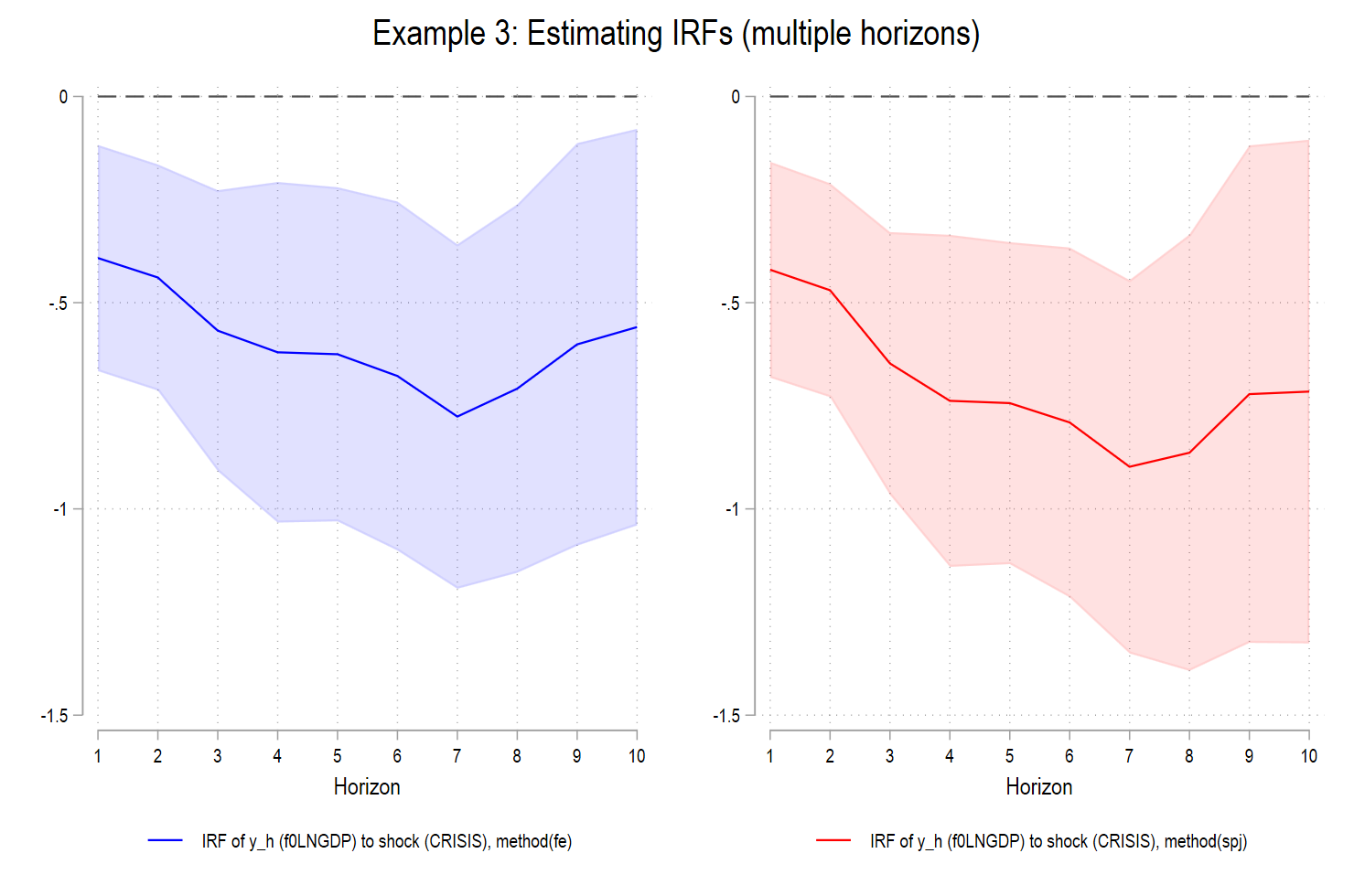
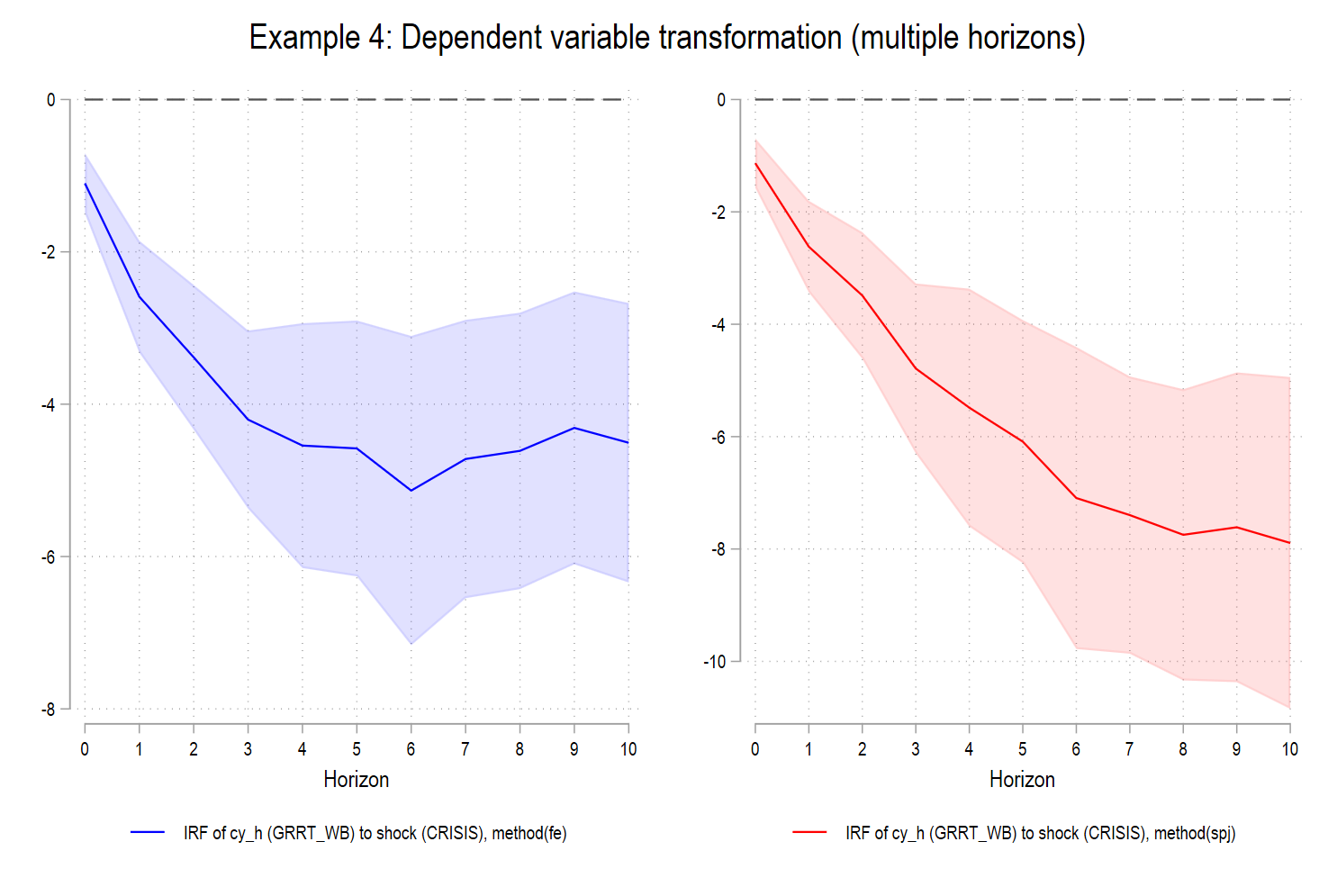
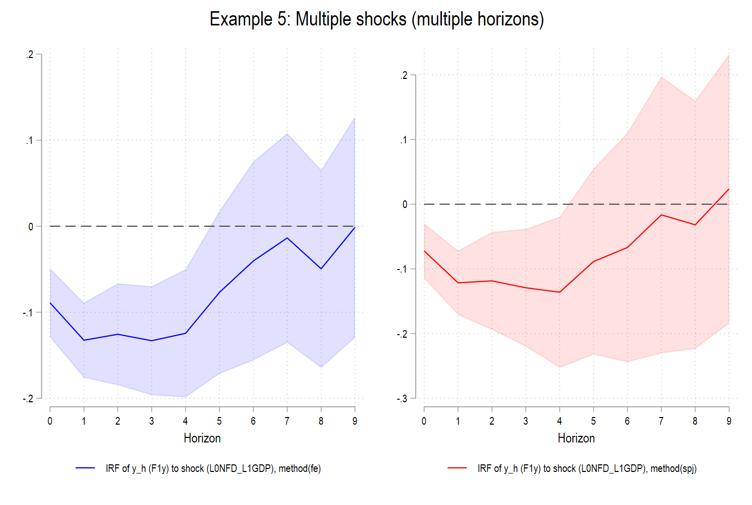
Across all applications in your output:

• FE-LP IRFs are systematically closer to zero at medium and long horizons.
• SPJ-LP IRFs display larger and more persistent responses, with wider confidence bands reflecting corrected uncertainty.
• The gap between FE and SPJ grows with the horizon; exactly as predicted by the theory.

This is not a cosmetic difference. It reflects the removal of a Nickell-type attenuation bias induced by fixed effects in predictive regressions.

8. Final takeaway

Panel local projections are powerful. When estimated with fixed effects, they rely on orthogonality conditions that fail in dynamic environments. The resulting Nickell-type bias can materially distort inference, especially at longer horizons.

The split-panel jackknife provides a clean, implementable correction that preserves the LP framework while restoring valid inference.

This is precisely the sense in which:

Panel LPs are robust to dynamic misspecification, but not to dynamic endogeneity under fixed effects. The SPJ correction solves this problem!

Appendix. Why dynamics break the FE orthogonality condition

Step 1 — What FE needs to be true (the target moment)

After demeaning, FE estimates the slope by OLS on

\tilde{y}_{i, t}=\rho \tilde{y}_{i, t-1}+\tilde{u}_{i, t},

where

\tilde{y}_{i, t}=y_{i, t}-y_i, \quad \tilde{y}_{i, t-1}=y_{i, t-1}-y_{i,-1}, \quad \tilde{u}_{i, t}=u_{i, t}-u_i .

For FE to be unbiased/consistent (for fixed $T$ and $N\to\infty$), we need the within orthogonality:

\mathbb{E}\left[\widetilde{y}_{i, t-1} \widetilde{u}_{i, t}\right]=0 .

Equivalently,

\mathbb{E}\left[\left(y_{i, t-1}-y_{i,-1}\right)\left(u_{i, t}-\tilde{u}_i\right)\right]=0 .

This is the condition that fails in dynamic panels.

Step 2 — Expand the condition and isolate the “bad term”

Expand the product:

\begin{aligned}
\mathbb{E}\left[\left(y_{i, t-1}-\bar{y}_{i,-1}\right)\left(u_{i, t}-\bar{u}_i\right)\right]= & \mathbb{E}\left[y_{i, t-1} u_{i, t}\right]-\mathbb{E}\left[y_{i, t-1} \bar{u}_i\right] \\
& -\mathbb{E}\left[\bar{y}_{i,-1} u_{i, t}\right]+\mathbb{E}\left[\bar{y}_{i,-1} \bar{u}_i\right] .
\end{aligned}

Now impose the standard dynamic-panel assumption that the shock is mean independent of the past (“predeterminedness” is enough here):

\mathbb{E}\left[y_{i, t-1} u_{i, t}\right]=0 .

Furthermore, under serially uncorrelated shocks, $\mathbb{E}[\bar y_{i,-1}u_{i,t}]$ is typically small and not the main driver. The key term is:

-\mathbb{E}\left[y_{i, t-1} \bar{u}_i\right],

Why is this term problematic? Because because \bar u_i contains u_{i,t-1}, and y_{i,t-1} contains u_{i,t-1}.

Step 3 — Show explicitly why $\mathbb{E}[y_{i,t-1}\bar u_i]\neq 0$

By definition,

\bar{u}_i=\frac{1}{T} \sum_{s=1}^T u_{i, s} .

Therefore,

\mathbb{E}\left[y_{i, t-1} \bar{u}_i\right]=\frac{1}{T} \sum_{s=1}^T \mathbb{E}\left[y_{i, t-1} u_{i, s}\right] .

Now split the sum into $s=t-1$ and $s\neq t-1$:

\mathbb{E}\left[y_{i, t-1} \bar{u}_i\right]=\frac{1}{T} \mathbb{E}\left[y_{i, t-1} u_{i, t-1}\right]+\frac{1}{T} \sum_{s \neq t-1} \mathbb{E}\left[y_{i, t-1} u_{i, s}\right] .

Under serially uncorrelated shocks and standard assumptions, the second term is approximately $0$. But the first term is not.

To see why, use the model itself at time $t-1$:

y_{i, t-1}=\mu_i+\rho y_{i, t-2}+u_{i, t-1} .

Multiply both sides by $u_{i,t-1}$​ and take expectations:

\mathbb{E}\left[y_{i, t-1} u_{i, t-1}\right]=\mathbb{E}\left[\mu_i u_{i, t-1}\right]+\rho \mathbb{E}\left[y_{i, t-2} u_{i, t-1}\right]+\mathbb{E}\left[u_{i, t-1}^2\right] .

Under the standard assumption that $u_{i,t}$ is mean independent of $\mu_i$ and the past, the first two expectations are $0$, leaving:

\mathbb{E}\left[y_{i, t-1} u_{i, t-1}\right]=\mathbb{E}\left[u_{i, t-1}^2\right]=\sigma_u^2>0 .

Thus,

\mathbb{E}\left[y_{i, t-1} \bar{u}_i\right] \approx \frac{1}{T} \sigma_u^2>0

This is the decisive fact.

Step 4 — Conclude: within orthogonality fails and the bias is order $1/T$

Return to the within orthogonality condition. The dominant term is

\mathbb{E}\left[\tilde{y}_{i, t-1} \tilde{u}_{i, t}\right] \approx-\mathbb{E}\left[y_{i, t-1} \bar{u}_i\right] \approx-\frac{\sigma_u^2}{T} \neq 0 .

Therefore, the regressor in the demeaned regression is correlated with the demeaned error. OLS on the within-transformed equation is biased.

And crucially, the magnitude is proportional to $1/T$. This is why Nickell bias is an incidental-parameters bias of order $1/T$.

Intuition (strictly consistent with the derivation)

• In the original model, $y_{i,t-1}$​ is uncorrelated with $u_{i,t}$​ (one-step-ahead exogeneity).
• FE replaces $u_{i,t}$​ with $u_{i,t}-\bar u_i$.
• The time average $\bar u_i$ contains $u_{i,t-1}$​.
• But $y_{i,t-1}$​ contains $u_{i,t-1}$​.
• Hence $y_{i,t-1}$​ becomes correlated with $-\bar u_i$, creating bias.

So FE doesn’t “create” endogeneity out of nowhere; it imports past shocks into the current error term through the demeaning operation.