The positional average known as the skewness allows you to assess the symmetry of a distribution. When the skewness is to zero, then the distribution is symmetric. You have 50% of the observations below the mean and 50% of the observations above the mean. Generally, the mean will be equal to the median.
As you may know, they are several formulas to compute the skewness (Cicchitelli et alli, 2021, chapter 6). The terminology is rather confusing, and it may be useful to recall how Wolfram Alpha compute the skewness. I can use the notion of standardized central moment that we have seen in this previous blog on the kurtosis:
The first standardized central moment is equal to zero:
\begin{align*}
\tilde{\mu_{1}} & = \frac{\mu _{1}}{\sigma^{1}} = \frac{\mu-\mu}{\sqrt{E[(X-\mu)^2]}} \\
& =\frac{\mu-\mu}{(E[(X-\mu)^2])^{1/2}}=0
\end{align*}
The second standardized central moment is equal to one:
\tilde{\mu_{2}} = \frac{\mu _{2}}{\sigma^{2}} = \frac{E[(X-\mu)^2]}{(E[(X-\mu)^{2}])^{2/2}}=1The third standardized central moment is equal to the skewness:
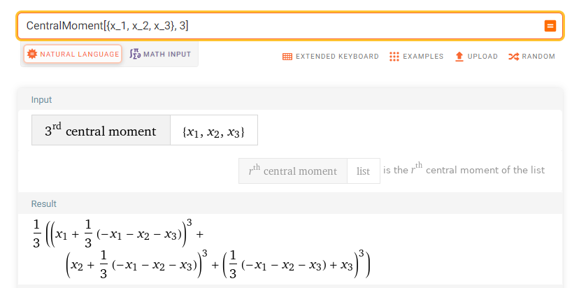
\tilde{\mu_{3}} = \frac{\mu _{3}}{\sigma^{3}} = \frac{E[(X-\mu)^3]}{(E[(X-\mu)^{2}])^{3/2}}=\text{skewness}As we can see on the following picture, with for a sample of three observations x1, x2, x3 (click on the images to have the Wolfram Alpha codes):
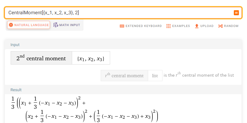
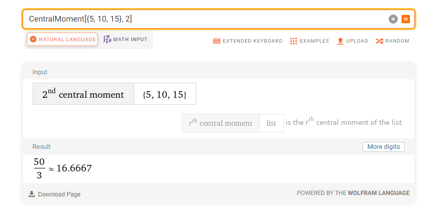
It may be useful to show how the second and third central moment are computed for the same sample:
Now, we compute the same moments, but with 3 numeric values for x1, x2, x3:
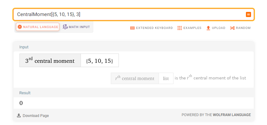
Of course, the skewness is zero in this pedagogical example since the distance between 5 and 10 is the same that the distance between 15 and 10:
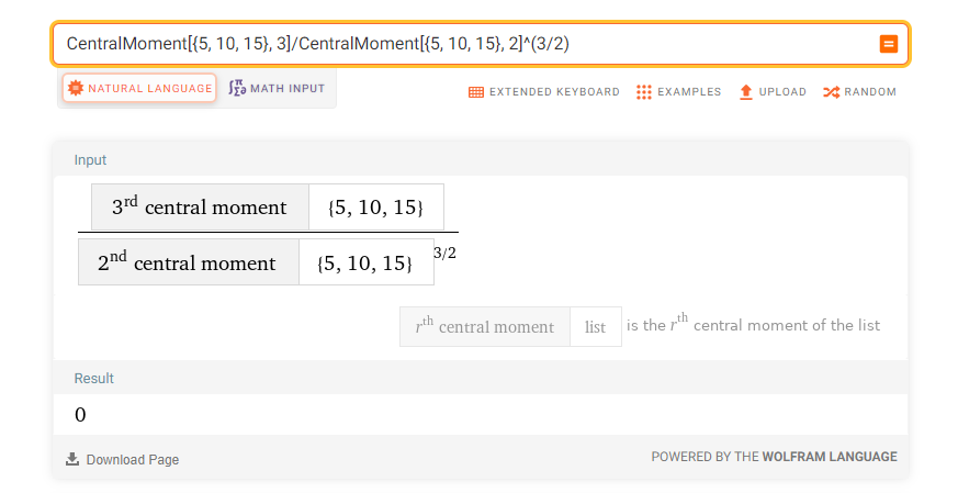
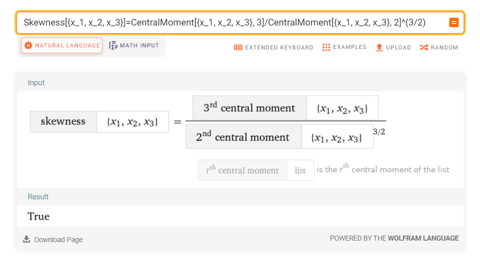
Finally, as it was to be shown, the last result is equal to the skewness’ formula based on central moments: