How to trace the growth effects of isolated treaty signatures in Stata

When countries sign several trade agreements in quick succession, a standard event-study can become hard to interpret. A coefficient estimated 2 years after one signature may already reflect the next signature. If the objective is to understand the dynamic effect of a single, clean treaty event, one useful strategy is to keep only isolated signatures.

This post shows how to do that in Stata with a simple local-projection-style event-study. The logic is straightforward: identify years in which the stock of agreements increases, keep only those events that are not contaminated by nearby signatures, estimate horizon-by-horizon regressions, and plot the dynamic response of growth.

The code below does exactly that.

1. The idea

Suppose eia is the cumulative stock of economic integration agreements. A new treaty signature is naturally proxied by a positive first difference:

$$\Delta eia_{it} = eia_{it} – eia_{i,t-1}.$$

A country-year is then classified as a signature year when $\Delta eia_{it} > 0$.

But this is not enough. If a country signs again 1 or 2 years later, the event window around the first treaty is contaminated. To deal with this, the code defines an isolated event as a signature that is not preceded by another signature in the previous 3 years and not followed by another one in the next 4 years. This matches the event-study window [-3,+4].

The goal is then to estimate a sequence of regressions of the form

$$y_{i,t+h} = \alpha_i + \lambda_t + \beta_h \, \text{isolated\_event}_{it} + \Gamma_h’ X_{it} + \varepsilon_{i,t+h},$$

for horizons $h=-3,-2,-1,0,1,2,3,4$, where:

• $y_{i,t+h}$​ is growth at horizon $h$,
• $\alpha_i$ are country fixed effects,
• $\lambda_t$​ are year fixed effects,
• isolated_event is the clean treaty-signature dummy,
• $X_{it}$​ contains controls, here lagged institutional capacity.

This is not exactly the same object as a full modern LP-DiD estimator, but it is a transparent and pedagogical way to visualize dynamic responses around isolated events.

2. Step 1: identify signature years

The first block creates the event indicator.

gen eia_change = D.eiagen sign_event = (eia_change > 0) if !missing(eia_change) ///
    & !missing(L.eia)
replace sign_event = 0 if missing(sign_event)

This simply says: a signature occurs when the stock of agreements rises.

3. Step 2: isolate clean signatures

The next step is the key one. We construct leads and lags of the signature dummy itself and keep only those signature years that are surrounded by zeros in the entire [-3,+4] window.

by imfcode: gen L1_sign = sign_event[_n-1]
by imfcode: gen L2_sign = sign_event[_n-2]
by imfcode: gen L3_sign = sign_event[_n-3]
by imfcode: gen F1_sign = sign_event[_n+1]
by imfcode: gen F2_sign = sign_event[_n+2]
by imfcode: gen F3_sign = sign_event[_n+3]
by imfcode: gen F4_sign = sign_event[_n+4]

foreach v in L1_sign L2_sign L3_sign F1_sign F2_sign F3_sign F4_sign {
    replace `v' = 0 if missing(`v')
}

gen isolated_event = sign_event == 1 & ///
    L1_sign == 0 & L2_sign == 0 & L3_sign == 0 & ///
    F1_sign == 0 & F2_sign == 0 & F3_sign == 0 & F4_sign == 0

This definition has a simple interpretation: keep only those treaties that look like standalone events within the event window.

That is often a good compromise between realism and interpretability. You lose some observations, but what you gain is a much cleaner event-study design.

4. Step 3: construct the horizon-specific outcomes

Instead of relying on a single event-study command, the code explicitly creates the dependent variable at each horizon:

gen y_m3 = L3.growth
gen y_m2 = L2.growth
gen y_m1 = L1.growth
gen y_0  = growth
gen y_p1 = F1.growth
gen y_p2 = F2.growth
gen y_p3 = F3.growth
gen y_p4 = F4.growth

This is a very transparent way to think about local projections.

• y_m3 is growth 3 years before the signature,
• y_0 is growth in the signature year,
• y_p4 is growth 4 years after the signature.

The event-study is then just a sequence of separate regressions, one for each horizon.

5. Step 4: estimate the horizon-by-horizon regressions

The code loops over the horizon-specific dependent variables, estimates a fixed-effects regression with clustered standard errors, and stores the coefficient on isolated_event.

local ctrls "L(1/3).INST"
local depvars "y_m3 y_m2 y_m1 y_0 y_p1 y_p2 y_p3 y_p4"
local hs     "-3 -2 -1 0 1 2 3 4"local i = 1

foreach y of local depvars {
    local hh : word `i' of `hs'    use `work', clear
    reghdfe `y' isolated_event `ctrls' if pop>2, ///
        absorb(imfcode period) vce(cluster imfcode)    use `irfstore', clear
    replace b = _b[isolated_event] if h == `hh'
    replace u = _b[isolated_event] + 1.96*_se[isolated_event] ///
        if h == `hh'
    replace d = _b[isolated_event] - 1.96*_se[isolated_event] ///
        if h == `hh'
    save `irfstore', replace    local ++i
}

So at the end of the loop:

• b contains the point estimate $\hat\beta_h$,
• u contains the upper bound of the 95% confidence interval,
• d contains the lower bound.

The controls here are L(1/3).INST, that is, 1 to 3 lags of institutional capacity. This is a reasonable choice if one wants to condition on slow-moving institutional fundamentals without loading the specification with too many covariates.

The if pop>2 restriction removes very small countries and may improve comparability.

6. Step 5: plot the dynamic response

The final graph uses vertical confidence bars and a connected coefficient line:

twoway ///
    (rcap u d h, fcolor(gs12) lcolor(gs12)) ///
    (connected b h, lcolor(black) mcolor(black) ///
        lwidth(medthick) msymbol(O) msize(small)), ///
    xline(-0.5, lpattern(dash) lcolor(gs8)) ///
    yline(0, lpattern(shortdash) lcolor(gs8)) ///
    xtitle("Years relative to isolated treaty signature") ///
    ytitle("Effect on growth") ///
    xlabel(-3(1)4) ///
    legend(off) ///
    graphregion(color(white)) ///
    plotregion(color(white)) ///
    note("Shaded area: 95% confidence interval. " ///
     "Average annual growth is about 0.039, so a coefficient of 0.01 corresponds to " ///
     "roughly 1 percentage point of growth.", ///
     size(small))

The dashed vertical line at -0.5 separates the pre-treatment horizons from the treatment year and the post-treatment horizons.

The horizontal line at 0 is the natural reference line.

The note is also useful. If average annual growth is about 0.039, then a coefficient of 0.01 is not trivial: it corresponds to roughly 1 percentage point of growth.

7. How to read the figure

The most interesting feature of this type of figure is usually the comparison between the pre-treatment and post-treatment parts.

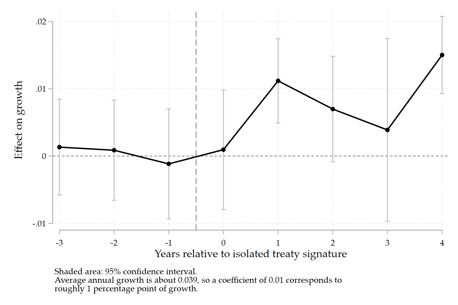
A convincing event-study pattern has 3 ingredients:

First, the coefficients before the event should be close to 0. This suggests the absence of strong pre-trends.

Second, the treatment year itself does not need to show a large effect. In many macro applications, one would actually expect the response to appear with delay.

Third, the post-treatment coefficients should display a pattern that makes economic sense. In this case, a gradual rise after signature is more plausible than an immediate jump.

That is precisely why isolating signatures is so useful. Without isolation, the dynamic path around one treaty can easily be polluted by another treaty just before or after it.

8. What this exercise is, and what it is not

This code is very useful pedagogically because it is transparent. Each horizon is estimated separately, and the researcher sees clearly how the dynamic profile is built.

But it is important to be precise.

This is:

• a local-projection-style event-study,
• estimated with reghdfe,
• around isolated treaty-signature events.

It is not a full LP-DiD estimator in the strict sense. So in applied work, I would present it as a complementary visualization rather than as the sole causal design.

That is also why it works well alongside a baseline LP-DiD specification. The event-study gives the picture. LP-DiD provides the more formal dynamic treatment-effect framework.

9. Full code

Here is the full block in one place.

**# Naoki style

// Run everything between preserve and restore (line 332-458)

preserve

cap drop eia_change 
cap drop sign_event 
cap drop isolated_event
cap drop L1_sign 
cap drop L2_sign 
cap drop L3_sign 
cap drop F1_sign 
cap drop F2_sign 
cap drop F3_sign 
cap drop F4_sign

gen eia_change = D.eia

gen sign_event = (eia_change > 0) if !missing(eia_change) ///
    & !missing(L.eia)
replace sign_event = 0 if missing(sign_event)

* Isolation rule matching window [-3,+4]
by imfcode: gen L1_sign = sign_event[_n-1]
by imfcode: gen L2_sign = sign_event[_n-2]
by imfcode: gen L3_sign = sign_event[_n-3]

by imfcode: gen F1_sign = sign_event[_n+1]
by imfcode: gen F2_sign = sign_event[_n+2]
by imfcode: gen F3_sign = sign_event[_n+3]
by imfcode: gen F4_sign = sign_event[_n+4]

foreach v in L1_sign L2_sign L3_sign F1_sign F2_sign F3_sign F4_sign {
    replace `v' = 0 if missing(`v')
}

gen isolated_event = sign_event == 1 & ///
    L1_sign == 0 & L2_sign == 0 & L3_sign == 0 & ///
    F1_sign == 0 & F2_sign == 0 & F3_sign == 0 & F4_sign == 0

tab sign_event
tab isolated_event

* Explicit horizon-specific dependent variables
capture drop y_m3 
cap drop y_m2 
cap drop y_m1 
cap drop y_0 
cap drop y_p1 
cap drop y_p2 
cap drop y_p3 
cap drop y_p4

gen y_m3 = L3.growth
gen y_m2 = L2.growth
gen y_m1 = L1.growth
gen y_0  = growth
gen y_p1 = F1.growth
gen y_p2 = F2.growth
gen y_p3 = F3.growth
gen y_p4 = F4.growth

tempfile work irfstore
save `work', replace

* Storage grid
clear
input h
-3
-2
-1
 0
 1
 2
 3
 4
end

gen b = .
gen u = .
gen d = .
save `irfstore', replace

local ctrls "L(1/3).INST"

local depvars "y_m3 y_m2 y_m1 y_0 y_p1 y_p2 y_p3 y_p4"
local hs     "-3 -2 -1 0 1 2 3 4"

local i = 1
foreach y of local depvars {
    local hh : word `i' of `hs'

    use `work', clear
    reghdfe `y' isolated_event `ctrls' if pop>2, ///
        absorb(imfcode period) vce(cluster imfcode)

    use `irfstore', clear
    replace b = _b[isolated_event] if h == `hh'
    replace u = _b[isolated_event] + 1.96*_se[isolated_event] ///
        if h == `hh'
    replace d = _b[isolated_event] - 1.96*_se[isolated_event] ///
        if h == `hh'
    save `irfstore', replace

    local ++i
}

use `irfstore', clear

twoway ///
    (rcap u d h, fcolor(gs12) lcolor(gs12)) ///
    (connected b h, lcolor(black) mcolor(black) ///
        lwidth(medthick) msymbol(O) msize(small)), ///
    xline(-0.5, lpattern(dash) lcolor(gs8)) ///
    yline(0, lpattern(shortdash) lcolor(gs8)) ///
    xtitle("Years relative to isolated treaty signature") ///
    ytitle("Effect on growth") ///
    xlabel(-3(1)4) ///
    legend(off) ///
    graphregion(color(white)) ///
    plotregion(color(white)) ///
	note("Shaded area: 95% confidence interval. " ///
     "Average annual growth is about 0.039, so a coefficient of 0.01 corresponds to " ///
     "roughly 1 percentage point of growth.", ///
     size(small))
graph export FIGURES\EVENTS_NAOKI.png, as(png) width(4000) replace

restore

10. Final takeaway

This code is a useful way to discipline an event-study when events are repeated and close together. The key contribution is not technical sophistication for its own sake. It is the simple idea that a treaty should be studied only when it is sufficiently isolated from other treaties.

That is often a very good instinct in applied macro and international economics.

If the researcher wants to understand the growth effects of a single treaty signature, isolating events first is typically better than pretending that all signatures are equally clean.